Note: Descriptions are shown in the official language in which they were submitted.
CA 02913945 2015-11-30
WO 2014/190414
PCT/CA2014/000460
- 1 -
Systems and Methods for Diagnosis of Depression and Other Medical
Conditions
Related Applications
[0001] This application claims the benefit of U.S. Provisional Patent
Application Serial No. 61/828,162 filed May 28, 2013, the entire contents of
which are hereby incorporated by reference herein.
Technical Field
[0002] The embodiments described herein relate to systems and methods
for diagnosing depression, and in particular to systems and methods for
diagnosis of depression based on analysis of sleep information.
Introduction
[0003] Human emotional states can generally be divided into two
categories (called mood and affective states) based on the persistence of each
state. Mood is generally considered to be a sustained emotional state that
lasts
for a few weeks or more. On the other hand, affective state (or affect)
generally
refers to a brief emotional response that is normally transitory in nature.
[0004] In general, affective responses are supposed to reinforce
behaviors
and serve important biological functions in mammalian physiology. However,
some of these affective responses, such as euphoria, depression and anxiety,
can become disturbed, persistent and dominant. When this happens, they can be
characterized as an illness or medical condition, and may require treatment.
[0005] Depression is a particularly problematic medical condition, and is
one of the most debilitating, costly, and stigmatized illnesses of our times.
It is
believed to affect an estimated 350 million people in communities all over the
world, and on average about 1 in 20 people have reported having an episode of
depression within the past year.
[0006] Unfortunately, notwithstanding the seriousness of depression, the
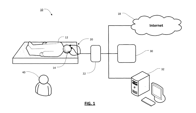
current techniques for its diagnosing and guiding treatment are generally
CA 02913945 2015-11-30
WO 2014/190414
PCT/CA2014/000460
- 2 -
inadequate. For example, depression may be diagnosed by reviewing the clinical
symptoms of a patient, such as by using the criteria contained in the
Diagnostic
and Statistical Manual of Mental Disorders (DSM-IV). DSM-IV is designed to
identify a mood disorder such as depression by examining three elements: mood
episodes, descriptors of most recent episode, and recurrence descriptors.
[0007]
However, the DSM-IV techniques are problematic, particularly since
examining these three elements requires input from the patients, including
their
ability to recognize and describe their own feelings. This ability can vary
from
patient to patient, especially for different cultural backgrounds, and tends
to
create inconsistencies in the results. Moreover, symptoms of depression can
vary greatly between different patients. As a result the DSM-IV method for
diagnosing depression tends to be subject to systematic error and often
results in
false results.
[0008] There
are some physiological tests that attempt to help diagnose
depression. Among these physiological tests are the dexamethasone
suppression test, the tyrotropin releasing hormone stimulation test, the
growth
hormone response to insulin-induced hypoglycemia test, and the plasma cortisol
level test. Unfortunately these physiological tests tend to be inconsistent
and may
be unreliable when used for diagnosis.
[0009] In
some cases, it may be possible to diagnose depression by
conducting a psychiatric interview of a patient. However, this approach tends
to
be heavily dependent on the abilities of the interviewer(s) and other factors
that
make it subjective and somewhat unreliable.
Brief Description of the Drawings
[0010] Some
embodiments will now be described, by way of example only,
with reference to the following drawings, in which:
[0011] Figure
1 is a schematic diagram illustrating a system for diagnosing
depression according to one embodiment;
CA 02913945 2015-11-30
WO 2014/190414
PCT/CA2014/000460
- 3 -
[0012] Figure 2 is a schematic diagram of a graphical user interface for
a
diagnosis system according to one embodiment;
[0013] Figure 3 is a schematic diagram of functional components of a
diagnosis system according to one embodiment;
[0014] Figure 4 is a detailed diagram of an analyzer module of a
diagnosis
system according to one embodiment;
[0015] Figure 5 is an diagram showing an example of sleep staging and a
corresponding digital period analysis (DPA) for two random samples according
to
one embodiment;
[0016] Figure 6 is an diagram showing an exemplary estimate of REM
density according to one embodiment;
[0017] Figure 7 is a schematic diagram of functional components of a
REM density estimator according to one embodiment;
[0018] Figure 7a is a diagram of an example of REM activity on EOG
channels;
[0019] Figure 8 is graph comparing beta bilateral coherency for adults
between a normal individual and a depressed individual;
[0020] Figure 9 is graph comparing beta delta coherency in the left
hemisphere for adults between a normal individual and a depressed individual;
[0021] Figure 10 is graph comparing beta delta coherency in the right
hemisphere for adults between a normal individual and a depressed individual;
[0022] Figure 11 is graph comparing theta bilateral coherency (TCOH) in
adults between a normal individual and a depressed individual;
[0023] Figure 12 is graph comparing beta delta coherency in the right
hemisphere for children between a normal individual and a depressed
individual;
CA 02913945 2015-11-30
WO 2014/190414
PCT/CA2014/000460
- 4 -
[0024] Figure 13 is graph comparing beta delta coherency in the left
hemisphere for children between a normal individual and a depressed
individual;
[0025] Figure 14 is an exemplary drawings of a model artificial neuron
according to one embodiment;
[0026] Figure 15 is an exemplary drawing of an artificial neural network
according to one embodiment;
[0027] Figure 16 is an exemplary drawing of an artificial neural network
according to another embodiment; and
[0028] Figure 17 is an exemplary graph of an estimate of coherence
according to one embodiment.
Description of Some Particular Embodiments
[0029] For simplicity and clarity of illustration, where considered
appropriate, reference numerals may be repeated among the figures to indicate
corresponding or analogous elements or steps. In addition, numerous specific
details are set forth in order to provide a thorough understanding of the
exemplary embodiments described herein. However, it will be understood by
those of ordinary skill in the art that the embodiments described herein may
be
practiced without these specific details. In other instances, well-known
methods,
procedures and components have not been described in detail so as not to
obscure the embodiments generally described herein.
[0030] Furthermore, this description is not to be considered as limiting
the
scope of the embodiments described herein in any way, but rather as merely
describing the implementation of various embodiments.
[0031] In some cases, the embodiments of the systems and methods
described herein may be implemented in hardware, in software, or a combination
of hardware and software. For example, some embodiments may be
CA 02913945 2015-11-30
WO 2014/190414
PCT/CA2014/000460
- 5 -
implemented in one or more computer programs executing on one or more
programmable computing devices that include at least one processor, a data
storage device (including in some cases volatile and non-volatile memory
and/or
data storage elements), at least one input device, and at least one output
device.
[0032] In some embodiments, a program may be implemented in a high
level procedural or object-oriented programming and/or scripting language to
communicate with a computer system. However, the programs can be
implemented in assembly or machine language, if desired. In any case, the
language may be a compiled or interpreted language.
[0033] In some embodiments, the systems and methods as described
herein may also be implemented as a non-transitory computer-readable storage
medium configured with a computer program, wherein the storage medium so
configured causes a computer to operate in a specific and predefined manner to
perform at least some of the functions as described herein.
[0034] As briefly described above, known methods for diagnosing
depression tend to be inadequate. In particular, existing diagnosis methods
tend
to be laborious, costly, subjective, time consuming, incomplete (i.e., they
may not
cover the full spectrum of the illness), or some combination thereof.
Moreover,
some known methods for diagnosing depression may be available only through
highly trained medical personnel (i.e., a psychiatrist), may not be easily
reproducible, and may be subject to error or very difficult to standardize.
[0035] At least some of the teachings herein are directed at systems and
methods for diagnosing depression which may provide for improved results as
compared to at least some previous known techniques.
[0036] Turning now to Figure 1, illustrated therein is a schematic
diagram
of a system 10 for diagnosing depression according to one embodiment.
[0037] In general, the system 10 may be operable for use in various
locations, such as a sleep clinic or laboratory, or other medical facility. In
some
CA 02913945 2015-11-30
WO 2014/190414
PCT/CA2014/000460
- 6 -
embodiments, the system 10 may be operable in another environment, such as
in a person's home.
[0038] Generally, the system 10 uses electroencephalography (EEG) to
monitor the sleep patterns of a patient (i.e. the patient 12 in Figure 1).
Electroencephalography (EEG) refers to recording measurements of electrical
activity along a patient's scalp. More particularly, an EEG measures voltage
fluctuations that result from changing current flows within the neurons of the
patient's brain.
[0039] An EEG can be useful for monitoring a patient's sleep patterns,
since brain function varies during waking and the different stages of sleep.
This
variation can be detected by the EEG. In particular, as a person sleeps their
brain generally switches between different stages of activity, with different
brain
wave patterns associated with each stage.
[0040] For example, stage 1 is the beginning of a sleep cycle, which is
relatively light sleep. During this stage, the brain produces alpha waves.
During
stage 2 sleep, the brain tends to produce theta waves, and can produce rapid,
rhythmic brain wave activity known as sleep spindles. In stage 3, which is a
transitional stage between light and deep sleep, the brain begins to produce
delta
waves, which are deep and slow. In stage 4, the brain is in a deep sleep and
produces many deep and slow delta waves. Depending on the particular sleep
classification system being used, in some case stage 3 and stage 4 sleep may
be grouped together and referred to simply as slow-wave sleep (SWS).
[0041] Finally, in stage 5, the brain enters Rapid Eye Movement (REM)
sleep, also known as active sleep. This is the stage in which the majority of
dreaming will occur.
[0042] As shown in Figure 1, to monitor the patient's 12 sleep patterns,
electrodes 20 of an electroencephalograph 22 (the EEG measuring device) may
be coupled to the scalp 14 of the patient 12 to observe brain wave activity.
CA 02913945 2015-11-30
WO 2014/190414
PCT/CA2014/000460
- 7 -
[0043] In some embodiments, the electrodes 20 could be placed onto the
scalp 14 using a conductive gel or paste. This technique may be particularly
suitable where the system 10 is being used at a sleep clinic or other medical
facility, and where another person 40 (i.e., a sleep clinician) may be
available to
assist with properly placing the electrodes on the scalp 14.
[0044] In some embodiments, the electrodes 20 could be located within a
cap or net that can then be placed on the head of the patient 12 so that the
electrodes 20 are properly positioned on the scalp 14. This approach may be
particularly suitable where the system 10 is being used at a person's home or
other similar environment, since it may allow the placement of the electrodes
20
on the scalp 14 to be controlled more easily, especially when a clinician may
not
be available to assist with electrode placement.
[0045] In general, brainwave information that is received via the
electrodes
20 may be processed by the electroencephalograph 22 to generate some sleep
data that is representative of the sleeping behavior of the patient 12.
Depending
on the particular configuration of the system 10, this sleep data may then be
sent
to one or more devices or diagnostic tools for analysis. In some cases, the
sleep
data may be in a raw state (i.e., generally unprocessed brainwave data). In
other
cases, the sleep data may be processed (i.e., converted to a hypnogram or
other
processed data).
[0046] In some embodiments, the sleep data from the
electroencephalograph 22 may be sent to a diagnosis device 30. The diagnosis
device 30 may for instance be a stand-alone device that is operable to
interpret
the sleep data and generate a depression diagnosis for the patient 12.
[0047] In some cases, this diagnosis may be done by the diagnosis device
30 without any intervention by a clinician or other user. In other cases, the
diagnosis device 30 may receive input from a user, for example to help
calibrate
CA 02913945 2015-11-30
WO 2014/190414
PCT/CA2014/000460
- 8 -
the diagnosis (i.e., to compensate for certain variables such as gender, age,
and
so on).
[0048] In some cases, the diagnosis device 30 may have dedicated
hardware components or software modules (or both), and may have various form
factors. For instance, in some embodiments, the diagnosis device 30 may be a
portable electronic device that may include a display screen, an input device,
a
power source, and other functional components. This embodiment may be
particularly useful where the diagnosis device 30 is adapted to be used in a
home environment.
[0049] In some cases, the diagnosis device 30 and electroencephalograph
22 may be provided as part of the same physical unit. For instance, the
diagnosis
device 30 and electroencephalograph 22 may have integrated hardware or
software components (or both) that are provided within a single unitary
housing
or body.
[0050] In other embodiments, the diagnosis device 30 and EEG measuring
device 20 may be separate and distinct, and may communicate in various ways,
such as by a wired or wireless communication channel.
[0051] In some embodiments, sleep data from the electroencephalograph
22 may be sent to a processing device 32 that is operable run a diagnostic
software application for diagnosing depression. In general, the processing
device
32 may be any suitable computing device, such as a server, personal computer,
laptop, tablet, smartphone, etc. In particular, the processing device 32 may
be a
general purposes computer running a software application that is designed to
interpret the sleep data and generate a diagnosis for the patient 12 therefrom
according to the teachings herein.
[0052] In general, the processing device 32 may include one or more
processors, one or more data storage devices, one or more input and output
CA 02913945 2015-11-30
WO 2014/190414
PCT/CA2014/000460
- 9 -
devices, and so on as will be suitable for controlling the operation of the
software
application.
[0053] In some embodiments, the sleep data from the
electroencephalograph 22 may be sent for analysis to a different location. For
example, the sleep data may be sent over the internet 18 or another
communications network to a diagnosis system that is remotely located from the
patient 12. This approach may be particularly- suitable where the patient 12
is
undergoing the EEG analysis at home, as it may allow diagnosis to be provided
as a service without requiring a diagnostic device to be physically present
with
the patient 12 and/or the electroencephalograph 22.
[0054] In some embodiments, as briefly discussed above, the sleep data
from the EEG measuring device 20 may be raw sleep data, such as measured
electrical activity related to the bra inwaves of the patient 12.
[0055] In other embodiments, the sleep data from the EEG measuring
device 22 may be processed to generate processed data (which might include a
hypnogram, for example) that is then sent to the diagnostic device 30, the
processing devise 32, and so on, so that the patient 12 can be diagnosed.
[0056] In some cases, raw sleep data can be automatically processed to
generate the processed sleep data, for example by a hardware or software
application designed to interpret EEG data and generate a hypnogram (or other
processed data) therefrom that shows various stages of sleep as a function of
time.
[0057] In other embodiments, the raw sleep data can be manually
processed (i.e., by the clinician 40 or other user) who may be trained to
interpret
raw EEG data and generate a hypnogram or other processed data.
[0058] Turning now to Figure 2, a schematic diagram of a graphical user
interface (GUI) 50 for a diagnosis system is shown according to one
embodiment. For example, the GUI 50 may be presented on the diagnostic
CA 02913945 2015-11-30
WO 2014/190414
PCT/CA2014/000460
- 10 -
device 30, on the processing device 32, as a web service (i.e., as a webpage
available over the internet 18), or in some other context.
[0059] In general, the GUI 50 may contain various controls and display
information that allow a user to perform a diagnosis on one or more patients.
For
example, the GUI 50 may contain a first display area 52 that shows information
about an EEG montage, and a second display area 54 that contains the results
of depression diagnosis for one or more patients.
[0060] The GUI 50 may also contain one or more progress indicators (i.e.,
progress bars 56, 58) that are indicative of the progress of one more aspects
of
the diagnosis, such as the analysis for a particular patient, the analysis of
a
group of patients, and so on.
[0061] The GUI 50 may also include controls for controlling the
diagnosis.
For example, one or more controls may allow a user to select a mode of
operation and load information from a particular file (i.e., a file that
contains sleep
data, such as raw sleep data or processed sleep data). In this embodiment, the
controls include a drop down list mode control 60 and a file open control 62.
[0062] Finally, the GUI 50 may also include other controls, such as
buttons
64, 66, that are operable for starting and stopping the diagnosis.
[0063] During use, a user may pick an input folder or file that contains
sleep data (i.e., using the file open control 62), and select a mode of
operation for
the diagnosis system from one or more particular modes (i.e., using the mode
control 60). In this embodiment, some of the modes include "Diagnose", "Load
Data from Files", "Train" and "Cross-Validation Test".
[0064] The Diagnose mode of operation may be the most commonly used,
and allows the GUI 50 to initiate diagnosis of a particular patient or
patients
based on sleep data that is loaded into the appropriate folder.
CA 02913945 2015-11-30
WO 2014/190414
PCT/CA2014/000460
-11 -
[0065] The Train mode may allow a user to create a different training set
that can be used for diagnosis, instead of various pre-computed diagnostic
templates that may have already been prepared for the diagnostic system.
[0066] The Cross-Validation Test may allow proper operation of the
diagnosis system to be checked, for example by running the diagnosis system
against a known reference set (i.e., a pre-computed or user created reference
set).
[0067] In this embodiment, the Load Data From Files is an auxiliary mode
that may be useful for adjusting the reference data set. In particular, it may
allow
synthetic data sets to be reused, and which are created prior to computing
diagnostic parameters, thus allowing a synthetic data generation process to be
bypassed.
[0068] When the Diagnose mode is engaged (i.e., by activating the start
button 64), the diagnosis system will look for any patient files in an
appropriate
input folder. If patient files are located, the diagnosis system can start
loading
data associated with these patients and begin its analysis. Current progress
may
be indicated by the progress bars 56, 58, which in this embodiment can show
progress both for the current patient being analyzed, as well as the overall
progress for a number of different patients.
[0069] As patients are analyzed, the second display area 54 can be
updated with results. For example, in one embodiment, the result for each
patient
might be displayed from the list of NO (meaning that the patient is not
depressed), YES (meaning that the patient is depressed), NOT TESTED (for
example if for some reason the patient was not able to be tested), or UNKNOWN
(if the diagnosis system cannot reach a definitive conclusion).
[0070] Turning now to Figure 3, illustrated therein is a schematic
diagram
of functional components of a diagnosis system 70 according to one
CA 02913945 2015-11-30
WO 2014/190414
PCT/CA2014/000460
- 12 -
embodiment. In general, these functional components could be executed in
hardware, software, or some combination thereof.
[0071] In general, the diagnosis system 70 includes an EEG reader 72 that
is operable to read sleep data files (i.e., the raw data files). In some
cases, the
EEG reader may decompress sleep data received from an
electroencephalograph (i.e., electroencephalograph 22) and then send this data
to a montaging block 75.
[0072] The montaging block 75 is operable to prepare the sleep data for
further analysis by an analyzer 78 as will be described in further detail
below.
[0073] In some embodiments, a user interface 74 may be used to control
one or more aspects of the diagnosis system 70. For example, the user
interface
74 may be the GUI 50 described above or some other suitable user interface.
[0074] In some embodiments, the diagnosis system 70 may include a
sleep report parser 76. When appropriate, the sleep report parser 76 may load
and extract relevant data from previously prepared sleep reports (i.e.,
existing
sleep reports for the patient 12), if such sleep reports exist and are
available.
These existing sleep reports may be analyzed and may in some cases be helpful
for determining whether the patient has any biological markers that are
associated with depression.
[0075] It should be noted that the use of existing sleep reports is not
required, and in some cases may be undesirable. In particular, prior sleep
reports
may have been prepared in different sleep clinics or laboratories, and
variations
in how each particular clinic prepares its sleep reports may impact the
consistency between prior sleep reports, potentially limiting their
usefulness.
[0076] Thus, in some cases, the diagnosis system 70 may be operable
without including any data from prior sleep reports, even when prior sleep
reports
are available. This may be done to avoid possible inter-laboratory variation
in the
sleep reports.
CA 02913945 2015-11-30
WO 2014/190414
PCT/CA2014/000460
- 13 -
[0077] In some cases, the diagnosis system 70 may be used without
receiving EEG data via the EEG reader 72, in which case the sleep report
parser
76 would be used to send only prior sleep reports to the analyzer 78. This
approach may be appropriate when a particular user wants to use his or her own
sleep staging and scoring, without generating any new sleep data. For example,
a sleep clinic may have already performed a number of sleep studies of a
particular patient, and may desire to use these existing sleep studies as the
basis
for a diagnosis.
[0078] Turning now to Figure 4, further details of an analyzer module for
a
diagnosis system 80 are shown according to one embodiment.
[0079] In this embodiment, the EEG reader 82 sends data to a pre-
processor 84, which is operable to prepare the sleep data for analysis (i.e.,
by
formatting the data as may be required for use by the analyzers and so on).
The
pre-processor 84 will then send this data to a montaging block 85 that
includes
one or more analyzers.
[0080] In this specific embodiment, the montaging block 85 includes three
analyzers: a microarchitecture analyzer 86, a sleep continuity and
architecture
analyzer 88, and a REM density analyzer 90.
[0081] The various analyzer modules 86, 88, 90 of the montaging block 85
may create a set of time series that characterize particular information about
the
sleep behavior of the patient 12, such as the patient's EEG data, eye
movements, and muscle tone levels during a particular sleep study.
[0082] These time series can then be sent to a transformer 92. The
transformer 92 in turn can convert the time series in a vector of parameters.
When properly tuned, the transformer 92 acts as an adapter between the
different data analyzers (i.e., the microarchitecture analyzer 86, sleep
continuity
CA 02913945 2015-11-30
WO 2014/190414
PCT/CA2014/000460
- 14 -
and architecture analyzer 88, and REM density analyzer) so that the data can
be
interpreted by a classifier 94 to render a diagnosis.
[0083] In general, the classifier 94 may be operable to build boundaries
between normal and depressed patients in a multidimensional state space.
Based on these boundaries, the classifier 94 can reach a binary decision about
whether the patient is or not depressed (i.e. the classifier 94 may generate a
YES
or NO answer about whether the patient 12 is depressed).
[0084] In some embodiments, instead of a YES or NO the classifier 94
may provide some indication of the severity of the depression (i.e., MILD,
MODERATE, SEVERE, etc.)
[0085] In some embodiments, the classifier 94 may provide other results
(e.g., UNKNOWN etc.) where it is unable to reach a definite conclusion in
regards to the depression of the patient 12.
[0086] In some embodiments, the decision boundaries of the classifier 94
are built from one or more training sets, and the patient that is being
diagnosed
(i.e., patient 12) is compared to pre-existing knowledge about normal
populations
to look for patterns associated with depression.
[0087] More specifically, it has been discovered that several sleep
related
characteristics are influenced by major depressive disorders (MDD).
Individually,
each of these sleep related characteristics may be inadequate as biological
sleep
markers of depression, since they may be subject to individual variability
between patients and hence may not be wholly reliable for an accurate
diagnosis.
[0088] However, by fusing a plurality of sleep related characteristics
together, it is believed that a multidimensional descriptor of the state of
the
patient can be defined, and which may be generally useful for diagnosing
depression in that patient. In particular, nonlinear classification methods
may be
CA 02913945 2015-11-30
WO 2014/190414
PCT/CA2014/000460
- 15 -
able to reliably separate depressed and normal subjects based on analyzing a
plurality biological markers.
Characterizing Sleep
[0089] Several methods of classification that integrate various aspects
of
sleep are chronobilogical, microarchitectural, macroarchitectural, and
continuity
of sleep, as will be discussed further herein. These characteristics are
modulated
by the presence of major depressive disorder (MDD).
Chronobiological markers
[0090] The sleep and wake states in humans and other mammals tend to
follow a cyclic pattern that is regulated by an internal circadian clock in
the
suprachiasmatic nucleus, a structure in the anterior hypothalamus. When
humans are removed from external cues, they will maintain an endogenous
periodicity of their circadian rhythm. In humans this period is slightly over
24
hours.
[0091] In addition to the 24 hour circadian rhythm, humans also
experience a rhythm with a shorter period called an ultradian rhythm (also
referred to as a sleep-wake cycle). One candidate biological marker for
diagnosing depression is a phase shift of the ultradian rhythm, which in
general is
described by an early REM stage.
[0092] In order to study the frequency spectrum of a very slowly evolving
phenomenon (like the ultradian rhythm), a sleep study for a particular patient
should contain at least one period of the periodic behaviour.
[0093] Since, the normal ultradian rhythm has a period of about ninety
minutes, a sleep record of at least 90 minutes long should be used. Indeed,
many sleep records are several hours in length (in some cases up to 8 hours in
CA 02913945 2015-11-30
WO 2014/190414
PCT/CA2014/000460
- 16 -
length or more), which should provide sufficient time to review the
variability in
the ultradian rhythm.
Continuity
[0094] The continuity of sleep may be measured in terms of the following
parameters that can be extracted from polysomnographic (PSG) studies. These
parameters include:
[0095] sleep latency (SL);
[0096] wake after sleep onset (VVAS0);
[0097] number of awakenings (NWAK);
[0098] sleep efficiency (SE);
[0099] and total sleep time (TST).
Macroarchitecture
[00100] The macroarchitectural abnormalities in sleep may include the
following parameters:
[00101] altered distribution of slow-wave sleep (i.e., patient lack the
traditional attenuation pattern across the night);
[00102] reduced slow-wave sleep (in minutes and/or percent);
[00103] decreased latency to the first episode of REM sleep (i.e. reduced
REM latency);
[00104] prolonged first REM period;
[00105] increased REM percent (if not REM time in minutes); and
CA 02913945 2015-11-30
WO 2014/190414
PCT/CA2014/000460
- 17 -
[00106] increased REM density (i.e. eye movements per minute of REM
sleep).
[00107] The altered distribution of sleep in depression was noted to have
resemblance to alterations observed due to aging (with the exception of REM
density, which is more or less invariable with age).
[00108] Conventional wisdom is that parameters like REM latency alone are
unsuitable as sleep markers indicative of depression. Thus, considering
architectural elements or continuity descriptors of sleep individual as
potential
sleep markers may be less promising than looking at the record as a whole.
However, by reviewing the sleep record as a whole, it is presently believed
that it
may be possible to provide a diagnosis of depression.
Microarchitecture
[00109] In addition to studying the diminution of delta wave amplitude and
incidence and increase in amplitudes in the beta band, the study of the
microarchitectuire of sleep employed a technique called digital period
analysis
(DPA) that allows for continuous measure of delta activity, as contrasted to
the
standard PSG technique where a specified proportion of an epoch (e.g., a 30
second epoch) has to be covered by delta activity, with variations being
artificially left out.
[00110] The coherence of EEG activity in various spectral bands appears to
provide significant results in discriminating between depressed persons and
controls. Further microarchitectural variables that may be indicative of
depression
are whole night beta and gamma activity during NREM (non-REM sleep), and
around sleep onset.
CA 02913945 2015-11-30
WO 2014/190414
PCT/CA2014/000460
- 18 -
[00111] In one case, the degree of association between sleep disturbance
and symptoms of depression were studied, and it was determined that sleep and
depression may be strongly related phenomena.
[00112] Relevant depression symptoms were found to be the core
symptoms of depression and not neurovegetative symptoms while on the sleep
side the relevant parameters were found to be mostly NREM variables.
[00113] The clinical relevance of sleep continuity disturbance appears to
be
that people with persistent insomnia have higher probability of developing
depression and those patients with no improvement of sleep continuity after
antidepressant treatment have higher chances of relapse than those with
improved sleep continuity.
[00114] The parameters related to the architecture of sleep are mainly REM
latency, REM density and SWS time. Out of these parameters it appears that
REM density may be correlated to severity of depression, particularly since
REM
latency can be a predictor of treatment outcome. More particularly, a reduced
REM latency is associated with poor treatment outcomes.
Coherence and Complex Coherency
[00115] The concepts of coherence and coherency will now be discussed.
Coherence may be used in various fields for time delay estimation, as a
measure
of linear relationship between two processes, for system identification, and
as a
measurement of signal-to-noise (SNR) power ratio. To clarify the difference
between coherence and coherency, the term "coherence" is the square of
"coherency".
[00116] In general, if a discrete stochastic process x is linearly related
to a
discrete stochastic process y, one can write:
G(f) = IH (f) I 2 Gxx (f)
CA 02913945 2015-11-30
WO 2014/190414
PCT/CA2014/000460
- 19 -
[00117] In this equation, Gyy is the power spectrum of the process y, Gxx
is
the power spectrum of process x, and H(f) is the transfer function. By
definition,
the cross power spectrum for this equation is:
Gxy = DFT(kxy)
[00118] where DFT is the discrete Fourier transformation operator, and kxy
is the covariance function between processes x and y.
[00119] Expanding the covariance and reversing the order of integration of
the Fourier transform and expectation gives:
G(f) = H(f)G(f)
[00120] Complex coherency is a function, defined as the ratio of the cross-
power spectral density of two random processes, and the product of their auto-
power spectral densities:
G(f)
Yxy = __________________________________
.\IGxx(f)Gyy(i)
[00121] The magnitude squared coherency, or "coherence", is bounded and
has support [0,11:
Cxy = y4
[00122] In a linear relationship, by inserting the first two equations
into the
equation for coherency, one gets Cxy= 1. As a first observation, it can be
noted
that the coherence can be interpreted as departure from a linear relationship
in
the case of two stationary random processes.
[00123] However, despite mentioning a linear relationship, this approach
is
not limited to linear processes. Any nonlinear process can be linearized to
some
extent, and the adequacy of such linearization can be evaluated. If a linear
model
is considered generally adequate (i.e., if it seems to be a reasonably good
CA 02913945 2015-11-30
WO 2014/190414
PCT/CA2014/000460
- 20 -
model), then the linear model can be used to provide valuable insight into the
particular process being examined.
[00124] In the case of performing an identification task of a stationary
process y, one can feed the process x into the input of a model, and then
adjust
the model by minimizing the least squares error between its output and the
process y. This yields a frequency characteristic of the model:
H(f) =
uxx
[00125] According to this equation, the frequency characteristic of the
model is related to the squared coherence by:
jGxx
C(f) = H(f)
yy
[00126] The model in signal processing literature is called a filter and
can
be characterized by a set of coefficients that uniquely describe the model.
This
suggests that the coherence can be interpreted as an optimal (or at least
desirable) normalized filter that minimizes (or at least greatly reduces) the
error
between the response of the filter to the process x and the process y. In a
case
of coherency, the model will describe the linear relationship between the two
processes, process x and process y.
[00127] The error between the estimate and the modelled process is itself
a
random process. The power of the error process between y and its estimate is:
Gee = Gyy(f)[1¨ Cxy(f)]
[00128] This means that for large coherence the error power is small,
whereas for small coherence the error power is large (depending on how much of
the y process is explained by its estimator model).
CA 02913945 2015-11-30
WO 2014/190414
PCT/CA2014/000460
- 21 -
[00129] The spectrum of a process can be considered as a sum of two
terms, a desired part and an error part:
Gyy = Gyy Cxy Gyy (1- Cxy)
[00130] The ratio of these components can be interpreted as either a
linear-
nonlinear power ratio, which is the fraction of power that is contained in the
linear
part of the relationship to the power contained in the nonlinear part of the
relationship. The other interpretation is as a signal to noise ratio (SNR),
which is
a ratio of the desired part relative to the undesired (noise) part of a model:
Gyy xy
Gee 1 ¨ Cy
[00131] Complex coherency can be further interpreted using spectral
representation theorem. According to this theorem a stochastic process can be
represented by:
x(t) = f eiwt dZx(co),
¨7r
[00132] where Zx is a another stochastic process, and for a given w, Z(w)
is a random variable. Describing each process as above, one then arrives at:
y(t) = f el' dZy(w),
¨7r
[00133] Using this representation it can be shown that the complex
coherency can be written:
cov(dZx (f),dZy(f))
cxy(f) = var( dZx(f))var(dZy(f))
[00134] From this equation, it can be observed that the complex coherency
can be interpreted as the correlation coefficient for the random variables of
the
component processes Z, of the two stochastic process x and y.
CA 02913945 2015-11-30
WO 2014/190414
PCT/CA2014/000460
- 22 -
[00135] C,w thus gives information on how x and y are linearly related. At
a
given frequency (f), C,v measures the relationship between the random
coefficients at a frequency f of two processes x and y.
Digital Period Analysis
[00136] Digital period analysis (DPA) will now be discussed. Sleep studies
often use the fractions of fixed time windows that include delta activity as
an
indication that a patient is in either stage 3 or stage 4 sleep. This is
related to
another form of signal analysis, called digital period analysis (DPA).
[00137] The frequency distribution of EEG waves is a multidimensional
random process. To analyze an EEG, time can be discretized into units of 30
seconds called "epochs". At a specific time (i.e., once in every 30 seconds),
the
EEG data will provide a stochastic distribution of frequencies, each
representing
a multidimensional random variable. (e.g., the distribution of delta waves at
some
time t is a one dimensional random variable, and the time evolution of a
distribution of delta activity is a one dimensional random process).
[00138] Extending this principle to the multivariate case, and sectioning
the
stochastic process at time t, a momentary frequency distribution can be
obtained.
This distribution can then be partitioned into the sub-bands of the different
brain
waves of interest: delta (1-4 Hz), theta (4-6 Hz), and beta (16-32 Hz).
[00139] The multidimensional random process is a simplified model of
sleep, similar to the relationship between an object and its shadow on a wall.
The
random process is expected to contain a strong ultradian component in
concordance with the known ultradian variation of sleep, similar to the shadow
preserving some resemblance to the original object.
CA 02913945 2015-11-30
WO 2014/190414
PCT/CA2014/000460
- 23 -
[00140] It is generally possible to study the variation of each of the one
dimensional random processes in isolation, in which case the
interrelationships
between various variables could be ignored.
[00141] On the other hand, a multivariate approach could be used that
includes possible interactions between the processes. This multidimensional
approach is believed to provide more meaningful results. In particular,
including a
number of interactions (in some cases, as many interactions as possible) may
provide a more complete picture of sleep and better distinguish "normal" sleep
from the sleep of a depressed person. These interactions can characterize the
slipping of one ultradian, random component relative to some other one-
dimensional ultradian random component of sleep.
[00142] A delay or advance of ultradian rhythms through modified REM
latencies is believed to be useful for diagnosing depression. It is therefore
helpful
to determine if the degree of slipping of a one-dimensional random processes
is
coherent, or if it is accompanied by some dispersion, or frequency dependent
slipping. In some cases, characterization of the dispersion of ultradian
rhythms
may also be a biological marker of depression.
[00143] In current sleep medicine practices, the analysis of sleep studies
is
usually performed in 30 seconds epochs. As part of standard methods of sleep
staging, some stages of sleep are identified by using proportions of waves of
a
specified duration and amplitude. Instead of using continuous proportions, a
fixed
threshold may be applied; a particular epoch may be either sub-threshold or
above this threshold and consequently called stage 3 or 4 accordingly.
[00144] The proportions of specific types of waves are informative of the
characteristics of sleep. Using proportions can be considered a more accurate
alternative for characterizing sleep as opposed to methods of power spectral
analysis.
CA 02913945 2015-11-30
WO 2014/190414
PCT/CA2014/000460
- 24 -
[00145] In particular, due to the fact that power spectral analysis is an
averaging method, and due to the loss of phase information, the power spectrum
(unlike the Fourier transform) does not preserve a one-to-one relationship to
the
original signal. As a consequence, the original signal cannot be restored from
the
power spectrum, and there can be different waves that have the same power
spectrum.
[00146] In some cases, it would be helpful to have an accurate measure of
the proportion of waves of different durations, as in a rolling distribution
of waves
in various frequency bands. To this end, a method of counting waves tends to
be
more suitable than the averaging method of power spectral analysis because of
the closer relationship between spectral content and the original time-series.
[00147] According to some of the teachings herein, a specific wave has a
duration and a corresponding frequency. Each specific wave is considered
either
to be in one band or another, and the sum of the duration of the waves is
equal
to the duration of the original time-series. This method is generally called
Digital
Period Analysis (DPA).
[00148] A variation on Digital Period Analysis (DPA) will now be
described,
where variations exist based on the filtering applied prior to segmentation
and the
segmentation method, with the goal of identifying possible wave boundaries.
[00149] In one example, samples of random processes were filtered with a
digital band-pass Infinite Impulse Response (IIR) filter with -100db/dec and
pass-
band (0.5Hz, 70Hz). A digital band-stop filter was also used for the line
frequency. The band stop filter was created using a High-Pass filter with
transition band (0.1, 0.5Hz) with ¨ 100db/dec and a Low-Pass filter with
transition-band (70, 80Hz) ¨ 100db/dec.
[00150] The filtering operation transformed the data in a zero mean random
variable. Original data is denoted on the two channels of interest x1 and x2
respectively. Each channel had a four dimensional sample of the random
CA 02913945 2015-11-30
WO 2014/190414 PCT/CA2014/000460
- 25 -
process. A section through the process at discrete time n, will be represented
by
the random vector:
x = [ns no no]
[00151] The significance of the random components will become clear as
the computation is undertaken. The computation of ni where i E (8, 0,13)
proceeds as follows. First, define the operator that finds the zero crossings
of a
time series:
zx = Zero(x) = tnix[n ¨ 1] * x[n] 01
[00152] where x is a random variable. Then define the derivative
operator
D:
Dx = x[n] ¨ x[n ¨ 1]
[00153] Using the operators D and Z, build the following random
processes:
fs
no= (ZX[i] ¨ ZX[i ¨ ¨4) ( zx[i] ¨ zx[i ¨ 1]
zx[i] zx[i ¨ 1]
fs) ________________________________ fs
[00154] which represents counting the waves that have a frequency in
the
delta range (i.e., 1-4Hz). One can then build the set:
zdx = Zero(Dx),
[00155] and define the following two random processes:
n o = Ei (zdx[i] ¨ zdx[i ¨ 1] f) (zdx[i] ¨ zdx[i ¨ 1] < fs )zdx[i] ¨zdx[i-
1]
7 4 fs
n o = Ei (zdx[i] ¨ zdx[i ¨ 1] ) * (zdx[i] ¨ zdx[i ¨ 1] <
32
fs )zdx[i] ¨zdx[i-1]
16 fs
CA 02913945 2015-11-30
WO 2014/190414
PCT/CA2014/000460
- 26 -
[00156] An exemplary illustration of sleep staging 110 and samples of the
no and no processes is presented in Figure 5, namely n6 (shown as the middle
graph 112) and no (shown as the lower graph 114). The ordinate represents the
percentage of an epoch covered with waves from the corresponding random
process.
[00157] In order to compute estimates of coherence, estimates of auto
spectra and cross spectra can be computed. For instance, one method is to use
an overlapped fast Fourier transform. However, due to resolution in the range
of
about 18.5 mHz, long samples are generally needed and this method is not
particularly suitable due to the limitations given by the sleep record
duration.
Another method amenable to short samples is the smoothed periodogram
method:
Gxy(e) -- ¨ 2)12W (2)d 2
--n-
[00158] where W is odd-length symmetric window, N is the width of the
window, and X is the power spectral density of the process x. This equation is
easier to compute in time domain:
Gõ = rim kõ[n]w[n]e with
N-1-1n1
1
k[m]= ¨N 1 x[i]x[i + Inl]
o
[00159] A further simplification arises due to the relation between
convolution and cross-covariance:
kxy = x*[¨n] * y[n] and similarly
kxx = x*[¨n] * x[n]
[00160] where, x* is the complex conjugate of x. Combining these
equations, one gets the computational relations:
CA 02913945 2015-11-30
WO 2014/190414
PCT/CA2014/000460
- 27 -
Gõ(0) = IDFT((x*[¨n] * x[n]) w[n])I
Gx3,(9) = IDFT( (x[n] * y[n]) w[n]) I
[00161] These can then be used to get the computational relation for C.
IFFT( (x*[¨n] * Y[n]) w[nDlIF FT ( (x[n] * Y[n]) w[n]) I
C, = IFFT((X* [-n] * x[n]) w[n])lIFFT((Y[¨n] * Y[n]) w[nD
[00162] In particular, the modulus was used due to the linear phase
introduced by the fast Fourier transformation employed in order to compute the
DFT (which assumes causal sequences).
[00163] Coherence is a random process, and the coherence Cõy is related
to a correlation coefficient and therefore follows the same distribution. As a
consequence applying a Fisher z-transformation will normalize the process:
zji = tanh-1(1Yii(01)
[00164] Based on this transformation, it is possible to compute confidence
limits for Cu:
tanh(zu ¨ b ¨ o-,Zo.5a) y tanh(zii ¨ b + 5zZ0.5a)
[00165] where Za is the 100a percentage point of the normal distribution
and
b= n ¨ 2p
[00166] p is the number of input processes that are linearly combined to
obtain a process y. Here, with one input and one output, p = 1 and b = (n-2)-1
(where n is the number of degrees of freedom). In this example the size of the
sample was approximately 1000 for 8.3 h of sleep.
[00167] Due to the fact that d.f. >> 2, b = n-1, For a = 0.05 one gets
with
Z0.025 = -1.9599 and
CA 02913945 2015-11-30
WO 2014/190414
PCT/CA2014/000460
- 28 -
az = (1 ¨ 0.0041.6Yij2+0.22)
1 1
tanh ¨ -N- ¨ 1.96a-z) y tanh(zii ¨ ¨N + 1.96az)
[00168] As an example having C = 0.8, one gets the 95% confidence
interval:
tanh (tanh.-1(3) ¨ ¨ (1 ¨ 0.0041.6*0.8+0.22)
y
1000 1000
tanh (tanh-1(V0.08) ¨ ¨1 + 1.96 (1 ¨ 0.0041.6*0.8+0.22)
1000 1000
REM Density
[00169] Turning now to Figure 6, illustrated therein is an exemplary
diagram
of an estimate of REM density according to one embodiment.
[00170] In general, a REM density estimator may work in conjunction with a
sleep analyzer module. In particular, the REM density estimator can detect the
rapid eye movement (REM) of a patient during sleep. This result can be refined
later on using sleep staging information.
[00171] In some cases, all of the REMs detected during stages other than
stage 5 (REM sleep) will be discarded (i.e., any detected rapid eye movements
associated with sleep in stages 1-4 will be ignored), which should help
provide
for a more accurate determination of REM density.
[00172] In some cases, the data is then filtered with a band-pass filter
with
pass band boundaries (0.5, 10 Hz) and a notch filter, so as to create a zero-
mean time-series.
[00173] Figure 7 shows a schematic diagram of some functional
components of a REM density estimator 130 according to one embodiment. In
CA 02913945 2015-11-30
WO 2014/190414
PCT/CA2014/000460
- 29 -
particular, this embodiment includes a first digital filter 132 that is
coupled to a
segmentation module 134. The REM density estimator 130 also includes a
synchronization analyzer 136, and is coupled to a second digital filter 138.
[00174] In some cases, the input channels for the REM density estimator
130 are either Electro-oculogram channels (EOG) or Fronto-Parietal (FP) EEG
channels. Eye movements will normally produce opposite polarity signals in the
two EOG channels. Confounding frontal slow activity will either have same
polarity or misaligned waves in the two EOG channels.
[00175] The segmentation module 134 is adapted to identify candidate
wavelets. The synchronization analyzer 136 then retains those candidates that
are aligned in opposition on the two EOG channels.
[00176] The segmentation module produces two series of vectors of the
form:
REMvUD,[k] =[A1 d11 dl2tJT
SYNCv,[k] = [v1 v2 v3ir
[00177] REMvUD contains important morphological characteristics of
wavelets: amplitude, duration of first half (d11), second half (d12) and time
of
occurrence (t). The input time series for segmentation are all zero-mean.
[00178] For this particular example, the noise level in the study was
first
estimated, and then the index set was built. Then an operator was defined that
finds the zero crossings of a time series x[n]:
zx = Zero(x) = {nix[n ¨ * x[n] 0}
[00179] Defining the derivative operator D as:
Dx = x[n] ¨ x[n ¨ 1]
[00180] and using the operators D and Z, the following random processes
can be built:
CA 02913945 2015-11-30
WO 2014/190414
PCT/CA2014/000460
- 30 -
fs
n 6 = (z[i] - Zx[i -1] ¨4) ( zx[i] ¨ zx[i ¨1]
z[i] ¨ zx[i ¨ 1]
is)
fs
[00181] which is actually counting the waves that have a frequency in the
delta range (i.e., 1-4 Hz). The set was then built:
zdx = Zero(Dx),
[00182] along with the set:
A = { x[ zdx[ n ] ] - x[ zdx[ n-1 ]] I zdx[ n]] - zdx[ n-1]] <= 0.2fs }
[00183] Let: N = card(A). The rank operator is then defined:
AopW [n] = p th rank of { A[0] ... A[ NI] }
[00184] where W is a window W = (0 1.. card(A)). Let p = 0.9*N, then define
the noise:
noiseA = AopW[n]
[00185] Setting the amplitude threshold:
* noiseA ; 2 * noiseA > 201
thr =
(2 20 otherwise
[00186] allows the following set to be built::
zx = Zero(x),
M = max(x) ; x E [ zx[n-1], z[n] ], n c [1, card(z)l
m = min(x) ; x [ zx[n-1], zx[n] ]
[00187] A vertex direction can then be defined:
Vup = M > Iml ? true : false;
[00188] In general, a wavelet is pointing up if between two consecutive
crossings of the baseline, a maximum point is larger than the absolute value
of a
CA 02913945 2015-11-30
WO 2014/190414
PCT/CA2014/000460
- 31 -
minimum point. This property is true due to the zero-mean property of the time-
series. Usually the most accurately identifiable point of the triple (V, Vi+1
V1+2) is
the vertex (V1+1).
[00189] A wavelet can be modelled by a triangle (V, V1+1 V,+2), and the
wavelet parameters are the signed amplitude and the durations of the half-
wavelets:
Al = x[ z,[i+1] ] - x[ z[i] ]
dl 1 = 101t3*(z.[i+1] - z,[i])/fs
d12 = 10^3*(zk[i+2] -
t = zx[i];
[00190] A candidate wavelet is detected when the characteristics meet
certain criteria:
REMvUDkj = { [A dl 1 d12 t]kj,T I dl 1 <d12; dl l+d12 >200; A> thr}
[00191] REMvUDki, represents the characteristic vector for REM "I" in
epoch
"j" on channel "k". A second set can then be built:
SYNCvki = { [zk[i] zk[i+1] z4i+2]]kj,T I dl 1 <d12; dl 1+d12 >200; A> thr}
[00192] where SYNCvkj, represents the synchronization vector for REM "I"
in epoch "j" on channel "k".
[00193] Figure 7a shows an example of REM activity on EOG channels. For
instance, the synchronization analyzer takes the sets SYNCvk where k = {1,2}
on
the two EOG channels and correlates their position as follows:
REM] = ft I StageREM[j] * SYNCviii [2] * (I ¨ SYNCv2ind < 100) *
(REMvUDiji [0111EMvUD2jni [0] <0) * _____
REmvuDip[o] <' * (REmvuD,,,õ[o] <4
REmvuD,,,T,[o] REmvuDili[o]
CA 02913945 2015-11-30
WO 2014/190414
PCT/CA2014/000460
- 32 -
[00194] The indices are as follows: j (epoch) I, m(index within epoch for
channels 1 and 2 respectively)
[00195] StageSREM is a boolean function that is true if the epoch is part
of
a REM stage. The stage may be provided by a stager module (not shown).
[00196] Each epoch has a set {REMi} of times where a REM occurred. In
this case, the whole study has a set of sets of REMS; one REM set for each
epoch "j" {RENA}, REMi is a set of REMs in epoch "j".
[00197] One can estimate the REM density in multiple ways depending on
the desired purpose. For instance, a rolling window of variable duration may
be
used, depending on the length of the REM episode.
E.2 m StageREM(k ¨ i) * Card(REMk)
RD[k] = ________________________________________________
StageREM(k ¨ i)
1--2
[00198] Setting M=1, one gets the REM count per epoch. Setting M to
sup(Card(REM;)), where sup stands for supremum, one gets the average REM
count per REM episode, where the duration of the REM episode can be anything
between 1 and 200 epochs.
Transformer
[00199] Various factors that can influence the architecture of sleep
include
the gender and age of a patient. For example, information about the evolution
of
normal sleep with age and gender can be obtained from various sleep clinics,
such as the Sleep and Alertness Clinic (Toronto), and is generally discussed
as
the ontogeny of sleep stage percentage.
[00200] Before classification by a diagnosis system, it may be beneficial
to
try to compensate for this variable bias (for example using the transformer 92
shown in Figure 4) to at least partially mitigate the effects of gender, age,
and so
CA 02913945 2015-11-30
WO 2014/190414
PCT/CA2014/000460
- 33 -
on. In order to correct for some such variability and distinguish
pathognomonic
signs, the following transformation of the sleep markers was adopted SM =
{TS1,
TS2, TSD, TREM}. The initial T or TS reads total and total stage respectively.
(SM ¨ SMF) + (1 F) *(SM ¨ SMm)
SM = F * ________________________
SMF SMm)
[00201] Where SMF bar represents average sleep marker for females of the
age group that bracket test cases. For example, for a female patient, age 45,
with
30% S2 we would obtain for SM = TS2:
TS2 = 1 * (30 ¨ 54) + (1 1) * (30 ¨ 54.75 54.75) __ = ¨0.44
54
[00202] The units after normalization are in the range [-1, 1], where
negative values are for cases with less than normal average sleep markers, and
positive values represent values that are above normal. The absolute values of
SM variables are generally in the range [0, 11.
[00203] Some classification methods include parameters that have close
ranges and similar variance. This is the case for multivariate distance
calculations.
[00204] Other parameters were normalized due to largely different ranges
as follows: sleep efficiency (SEE), arousal index (ARI), sleep onset (SO), REM
latency (REM_LAT), apnea-hypopnea index (AHI), periodic leg movements
(PLMS), age (AGE), number awakenings (NUM_AWA), lights out to sleep onset
(LOSO), total sleep time (TST), wake after sleep (WAS), sleep period time
(SPT)
as follows:
[00205] SEF = SEF/100;
[00206] ARI = ARI/1 00.0;
[00207] SO = SO/100.0;
[00208] REM LAT = REM LAT/120.0;
CA 02913945 2015-11-30
WO 2014/190414
PCT/CA2014/000460
- 34 -
[00209] AHI = AHI/100.0;
[00210] PLMS = PLMS/100.0;
[00211] AGE = AGE/100;
[00212] NUM_AWA = NUM_AWA/100;
[00213] LOSO = LOSO/100;
[00214] TST = TST/1000;
[00215] WAS = WAS/1000;
[00216] SPT = SPT/1000;
[00217] At this point all parameters have been calculated and normalized
and one can proceed to classification methods.
Classification
[00218] Before discussing the classification step in greater detail, it may
be
helpful to review some of the above described teachings.
[00219] In particular, a set of microarchitectural parameters may be
calculated that result from ultradian rhythm relationships. These parameters
can
then be adjusted for bias and variance.
[00220] Furthermore, a set of biological markers can be extracted based on
sleep architecture and a set of sleep continuity indicators (which may be
normalized). All absolute values can be normalized within the range [0, 1],
thus
setting the stage for multivariate classification in a [-1, 11 hypercube.
[00221] In general, there are numerous ways of classifying multivariate
data. The common denominator is that they are all statistical in nature. The
next
task is thus a binary classification problem, to answer the question: is the
multivariate test vector in class A (normal) or B (depressed)?
CA 02913945 2015-11-30
WO 2014/190414
PCT/CA2014/000460
- 35 -
[00222] One of
the ways to solve the classification task is by using an
artificial neural network. A brief discussion of neural networks is provided
herein,
although it will be appreciated that neural networks are incredibly complex
and
powerful and a detailed discussion is beyond the scope of this document.
[00223] In
general, an artificial neural network is a machine that is designed
to model the way the brain performs a particular task. A neural network is
formed
by using artificial neurons connected by synapses in ways mimicking the
biological neuronal network model. Examples of a model artificial neuron and
artificial neural network are shown in Figures 14 and 15, respectively.
[00224] In
general, artificial neurons are computational units that have a
variable number of input synapses that permit them to connect to other neurons
in a network. The set of synapses of a neuron forms the receptive field of the
neuron. A synapse is characterized by its strength and is modified by exposing
the network to training patterns. Synapses can be inhibitory or excitatory.
Artificial neural networks are therefore considered to be knowledge encoders.
Knowledge is information used by the network to respond to exterior stimuli
applied to its receptive field.
[00225] The
synaptic inputs may be summed in an accumulator which is the
mathematical equivalent of the soma, or cell body of biological neurons. Thus,
the artificial neuron acts as a linear combiner:
Vk =
WkiXi
i=1
[00226] The
output of the linear combiner is called induced local field or
activation potential.
[00227] The
other ingredient of a neuronal model is the activation function,
which limits the output of the neuron to a finite value, thus making the
neuron a
CA 02913945 2015-11-30
WO 2014/190414
PCT/CA2014/000460
- 36 -
nonlinear computational element. For example, the function implemented by a
single neuron may be modeled as:
Yk = (P(IWkiXi bk
ti=-1
[00228] where bk is a bias, and if present can shift the input of the
neuron
up or down depending on its value.
[00229] Various kinds of activation functions may be used as are generally
known, such as sigmoid, hyperbolic tangent, and a Heaviside function
cp(v(n)) = a tanh( bv(n) )
1
(P(v) = 1 + exp(¨av)
[00230] In general, the hyperbolic tangent and the sigmoid functions are
continuous and therefore differentiable whereas the Heaviside function is not.
[00231] One specific example of a fuzzy logic method that may be
implemented will now be described. In this embodiment, a multilayer
feedforward
artificial neural network was created with one hidden layer and one output
layer,
also commonly called a multilayer perceptron and as generally shown in Figure
16.
[00232] This type of neural network is called a perceptron due to the
presence of the nonlinear activation function, and this type of network learns
with
a teacher. In particular, the repeated presentation of training examples
produces
an error signal at each neuronal output from the output layer.
e(n) = dj(n)¨ yi(n)
[00233] The error signal is the difference between the desired output (d)
and the actual output (y) at each time step (n).
CA 02913945 2015-11-30
WO 2014/190414
PCT/CA2014/000460
- 37 -
[00234] Assuming a batch mode of training the average error energy may
be computed as:
1 2
E=
n=1 W
[00235] The double summation is over all the synaptic weights (W) and all
presentations of training patterns (N). The adjustment of weights may be done
in
a direction opposite to the gradient of the error energy. This adjustment has
the
effect of decreasing the error energy and therefore bringing the output closer
to
the desired response:
aE
Am; =
owi;
[00236] The weight adjustment is generally done only after the network has
been presented the whole set of training patterns. This equation can thus be
expanded using the chain rule of differentiation and specifying the form for
the
activation function. In particular, the learning rate ri can be adjusted as
the
number of iterations increases.
[00237] The algorithm for training this network is general as follows
[00238] 1. Initialize network
[00239] Set the weights to values picked from uniform distribution with
zero
mean and variance, in order to set the standard deviation of induced fields of
neurons to be above the linear part and below the saturation part of the
activation
function. A simple and popular choice is initialization of weights from a
uniform
distribution is between -1 and I.
W,J= rand(-1,1)
[00240] 2. Train the network: forward pass
CA 02913945 2015-11-30
WO 2014/190414
PCT/CA2014/000460
- 38 -
[00241] Compute starting at the input layer, for each neuron the output
using linear combiner equation above. When all outputs of first layer are
available, compute the output of the second layer using as input the output
from
the previous layer.
(n) =1whyri
= o
[00242] where L is the layer number, j neuron from layer I, y, input on
synapse I of neuron j. The error between desired output and actual output on
neuron j is then:
e (n) = d j (n) ¨ (v j (n))
[00243] 3. Train the network: error back-propagation
[00244] Take the error from the output layer of neurons and propagate
toward the input in order to redistribute the blame for error among the
neurons of
the network. To do this, the gradients or the error energy should be computed:
dE (n)
V = ____________________________________
äw1(n)
[00245] Then the synapses can be updated:
a E (n)
Awii =
au ji(n)
[00246] and the local gradients computed for neuron j:
aE (n)
j (n) = _________________________________
a v (n)
[00247] There are distinct cases for neuron j being an output neuron (L2)
or
a hidden neuron (L1):
CA 02913945 2015-11-30
WO 2014/190414
PCT/CA2014/000460
- 39 -
a -
e .1 (n) _____________________________________ j L 2
av1(n)
81(n) = A
1+1 1+1
ok Wki (n) ;
ay! (n)
kcl, 2
(00248] For the activation potential of neuron j in layer I, one then
arrives at:
a cp b
ay! (n)
_________________________ = (a ¨ y 1 (n)) (a + Y1 (n))
a
[00249] Combining these equations allows the local gradient of neuron j in
layer Ito be determined:
(di (n) ¨ yj (n)) (a ¨ y (n)) (a + yj (n)) ; j eL2
[00250] 81(n) = a ,
j (a ¨ y( n)) (a + y; (n)) EkeL2 8171Wiliftl (n) ;
jE ¨1
a
[00251] 4. After all test examples have been exhausted update all the
weights for all the neurons using the stored history of partial derivatives
from all
training examples:
=A141 ¨ '11k1IN y( n)81 (n)
JL
I. n=1
[00252] In this equation y, is the input signal to neuron j on synapse I
at time
n.
[00253] Using this approach, there are generally two passes of the
computation for each training example: the forward pass, where the information
is propagated through the network and no modification is made to the synaptic
weights, and the backward pass, where the error signal between the desired
response and the actual response is redistributed in the network and
corrections
are made to the synapses based on the blame assigned to each neuron.
[00254] Various optimizations and training algorithms are generally
possible.
CA 02913945 2015-11-30
WO 2014/190414
PCT/CA2014/000460
- 40 -
[00255] For example, gradient descent with momentum sues a modification
of the update rule for synaptic weights based on previous updates:
Lm/j1(n) = c thwji(n ¨ 1) + 71Si (n)y i(n)
[00256] The momentum constant a has the role to avoid network instability
and has an absolute value between 0 and 1. It can be proven, by solving the
difference equation, that for consecutive, same direction variation of the
weight
vector accelerates the descent while for alternating sign changes it
decelerates
the descent on the error surface, thus stabilizing the learning. Practically
this is
not necessarily so. The momentum constant is a new problem dependent
parameter that doesn't seem to solve anything.
[00257] A Riedmiller algorithm has the advantage that besides adjusting
the
learning rate it eliminates the dependence on the partial derivative of the
error
energy which can be unexpected and therefore the whole adaptation of the
learning rate is vacuous.
[00258] In particular, the following values may be computed:
1 = 4_
71-61: j(fn ¨ 1) if ____________________________________ aa EE ( ,n) ¨aaE
E(n¨i) <0
ALi
awij awij
71 0. ¨ 1) i f ¨ o.) ¨ (n ¨ 1) > 0
Aij(n ¨ 1)
[00259] This equation may then be used to update the synaptic weights:
aE
¨Ai; if ¨ (n) > 0
Am; = aE
Au if ¨ (n) <0
awif
0
[00260] In this equation, weights are decreased if the error is growing
(partial derivative positive) and increased if the partial derivatives are
negative.
CA 02913945 2015-11-30
WO 2014/190414
PCT/CA2014/000460
- 41 -
[00261] In this approach, these equations are computed at the end of each
epoch, when all training patterns have been presented to the network. The next
epoch then uses the adapted values. Then another adaptation takes place and
so on and so on.
[00262] For each epoch, the data can be transformed to zero mean and
standard deviation 1:
x ¨
Y = ______________________________________
ElAxi ¨ x-)2
[00263] Next, one can de-correlate the inputs because correlations will
induce preferential learning directions. In order to achieve this goal, one
can use
the Karhunen-Loeve transform (KL). The KL transform finds linear combinations
of input variables that have maximal variance and zero covariance. This step
will
both reduce the redundancy of the variables by eliminating low variance
components and eliminate preferential learning directions. The KL transform is
obtained by projecting input vectors on the eigenvectors or the covariance
matrix.
[00264] In some cases, the low variance directions should be removed at
the 0.01 level.
[00265] The classification of a test vector is accomplished after applying
the
same transformation to the test vector that was applied during training,
namely
the test vector may be projected on the principal directions of the training
covariance matrix.
[00266] Generally, performance is influenced by network configuration,
complexity of the problem and adequacy of the training set. In some cases, it
may be beneficial that the network configuration should be the simplest that
is
capable of solving the problem.
[00267] One practical rule for selecting the number of training patterns
to
achieve a good generalization performance is 0 (W/c), where W is the number of
CA 02913945 2015-11-30
WO 2014/190414
PCT/CA2014/000460
-42 -
synapses in the network and is the maximum percent error accepted. (e.g.,
for
4 input parameters, 7 neurons in the hidden layer and 2 output neurons one
getsW = 4*7 + 7*2 = 42 N = 42/0.1 = 420).
[00268] By trial and error a network with 7 hidden neurons and 2 output
neurons was identified as being suitable for our application. The receptive
field of
the sensory neurons in the hidden layer was variable between 2 and 36 inputs,
depending on which parameters were discarded in our trials. The results are
presented in the discussion section below.
[00269] It will be appreciated that in general, various other
classification
techniques may be used accordingly to the teachings herein, and will not be
discussed in detail. For example, it may be possible to use a two layer neural
network which has Radial Basis Function (RBFNN) neural network as a first
layer. A RBFNN is a three layer neural network that has a layer of sensory
neurons, a hidden layer and a set of output neurons. This type of network
solves
the classification problem by treating the problem as a function fitting
problem in
high dimensional space.
[00270] Other types of neural networks that might be suitable for
classification include Probabilistic Neural Networks (PNNs), and Support
Vector
Machines (SVMs).
[00271] In some embodiments, it may be possible to use combinations of
weak models to obtain performance comparable to strong learning models using
committee machines. For example, one approach called bagging uses model
averaging, where a number of learning machines (experts) would be trained to
solve the classification problem. Other techniques include boosting by
filtering,
the AdaBoost algorithm, CART (classification and regression trees), using a
committee of logistic experts, using mixtures of experts (ME), and using a
hierarchical mixture of experts (HME).
CA 02913945 2015-11-30
WO 2014/190414
PCT/CA2014/000460
-43 -
[00272] In the particular classification problem being faced here, the
classifier must decide whether a vector x is from class C1 or C2. The
uncertainty
that characterizes the problem is summarized by the joint probability density
p(C,
, x), which is commonly known as inference. Once the inference step is
complete, decision theory can be applied to solve the classification problem.
[00273] Given a vector x, one would like to determine if a particular
patient
is depressed or not based on an available a training sample. Using Bayes'
theorem, the posterior probability can be determined as:
p (x I C (C1)
p(Cilx) =
p(x)
[00274] In the particular case we are interested in, namely a binary
classification problem, p(C) represents the prior probability for class C,
with the
probability to observe x:
p(x) = p(x I C1) + p(x I C2)
[00275] At the same time we have the joint probability:
p(x, C,) = p(x I C,)p(C,)
[00276] If a prior p(Ci) is available, then one can get a revised
posterior
probability due to the addition of the new information due to the latest test.
[00277] In general, the determination as to whether a patient is depressed
or not may be based in the maximum posterior probability.
[00278] Another aspect in decision theory is the minimization of the cost
due to error. This theory provides techniques for considering the risk
associated
with misclassification. In particular, the prevalence of disease in the
population
and asymmetrical risk associated with false positives and false negatives must
be considered.
[00279] More specifically, if population sample where the normal state is
prevalent is used to train a diagnostic system, then this data will
potentially
CA 02913945 2015-11-30
WO 2014/190414
PCT/CA2014/000460
-44 -
undersample the population of diseased cases and therefore provide incomplete
learning. Balancing the training populations, on the other hand, may create
false
priors due to the exaggerated presence of disease states within the sample
set.
Corrections should be made to adjust these priors to provide a training sample
that generally accurately reflects the distribution of depression within a
population.
[00280] For example, one can introduce a loss function L which is the
overall cost due to the incurred decisions. In some cases the goal is to
reduce
and even minimize E(L) by finding the regions R, that best accomplish that
aim:
E[L] = argmax f dx Ljip(x, Ci) =ILitp(Cj(x)
Ri
[00281] In this equation, R, is decision region for class C, given the
example
is from class C. The second equality in this equation results from Bayes'
theorem
and observing that p(x) doesn't participate in the maximization.
[00282] This can be done by knowing the posterior probabilities. In
particular, priors p(C1) can be computed from the training set as well as the
class
conditional densities. Decisions can then be made by using the maximum
posterior probability criterion.
[00283] In some cases, the cost function can be changed on the fly, for
instance based on application once the posterior probabilities were
determined.
In a clinical situation it may be more important to increase the sensitivity
of the
test for screening purposes, knowing that if a false positive is returned,
more
tests may be done to increase the specificity of the overall diagnostic (and
which
can correct for a false positive).
[00284] In another setting, if the clinician has already some evidence of
the
existing disease and wants confirmation from complementary tests, then the
clinician may choose to balance the cost in favor of specificity.
CA 02913945 2015-11-30
WO 2014/190414
PCT/CA2014/000460
- 45 -
[00285] In addition, in some cases decision zones with lower than desired
posterior probability can be excluded. For instance, in cases where posterior
probability is lower than a threshold can be considered as undecided.
[00286] In some cases, mixed information from different sources can be
divided and treated separately. The results can then be combined using
probability theory. For example the parameters stemming from the
microarchitecture of sleep could be used independently (more or less
artificially)
from the more conventional sleep markers. In this case, the results may be
combined, during training, in class conditional joint probabilities:
ID(xm, xcl C1) = P(xml P(xcl C1)
[00287] In general, the posterior probability can be used to reach a
decision:
P (Ci J xm)P(Ci Ixc)
P (Ci I xnõx,) =
p(C1)
[00288] The priors P(C1) can be estimated from the proportion of the data
pertaining to each class in the training sample (assuming random sampling).
[00289] To reach a final determination on classification, various
techniques
may be employed. For example, one form of classification doesn't require
estimation of posterior probabilities and estimates the input-output
relationship
directly. A popular method minimizes the least square error between the model
and the desired output. The simplest discriminant (linear discriminant) builds
a D
- 1 dimensional hypersurface in a D dimensional decision space.
[00290] In other cases, probabilistic models based on maximum posterior
probability may be used. Furthermore, it may also be possible to use k Nearest
Neighbour (kNN) approach. The kNN approach has some very nice features that
make it desirable in some applications. Among the advantages are the
independence on distribution of the data in the decision volume, furthermore,
this
method is not disturbed by the uneven density of training data in high
CA 02913945 2015-11-30
WO 2014/190414
PCT/CA2014/000460
-46 -
dimensional spaces, a problem known as curse of dimensionality. Another
advantage is that the error of the method is never worse than twice the
minimum
achievable error rate.
[00291] Various other techniques for reaching a final determination on
classification will be appreciated based on the teachings herein.
Various Alternative Embodiments
[00292] In general, the teachings herein may be used in various different
embodiments that may be useful for diagnosing depression.
[00293] For example, in one embodiment, the teachings herein may be
implemented in stand-alone software. In particular, diagnostic software
application may be provided that can complement existing polysomnographic
equipment, for example as used in sleep laboratories and other medical
facilities.
In some such cases, the diagnostic software may be implemented using existing
hardware, such as a processing device already present in a sleep laboratory.
[00294] In general, assuming that sleep laboratories have equipment that
is
adequate for recording EEG, the teachings herein may be useful to provide
enhanced diagnostic methodology for sleep that can help diagnose depression.
[00295] In some embodiments, the teachings herein may be used to
provide an extra analysis of the sleep record and functions as a screening
tool for
depressed people in a sleep laboratory. This is in agreement with the
relatively
well known fact that about 20-30% of the patients seen for sleep disorders in
the
sleep laboratory are depressed and should be diagnosed and treated
accordingly.
[00296] In another embodiment, the teachings herein could be used to
provide a software application for use in a patient's home. This may include
using
a headbox that can be sent to a patient's home, and can be used in combination
with an EEG review station existing remotely at the point of care.
CA 02913945 2015-11-30
WO 2014/190414
PCT/CA2014/000460
-47 -
[00297] More particularly, currently the clinician in a sleep laboratory
will
analyze sleep stages using a well-established method that includes relatively
precise positioning of the electrodes on the scalp of a patient.
[00298] In a patient's home, there are several barriers to this approach.
First, it is generally not possible (or at least may be difficult) for a
patient to apply
the electrodes to his or her own scalp. Furthermore, most patients will likely
lack
anatomical knowledge that is necessary to achieve standard electrode
placements on a scalp.
[00299] Moreover, an additional barrier is one of interpretation. In
particular,
namely replacing the standard electrode arrangement that a clinician would use
means that one can no longer reliably use the textbook approach for
interpretation and thus would normally be unable to produce a reliable
diagnostic
based on the standard set of rules. More specifically, these rules tend to be
become highly unusable as electrode placement varies, since these are tightly
bound to the recording technique.
[00300] Some of the teachings herein are directed to new methods that
may overcome at least some of these difficulties, particularly for the home
setting, and yet still and provide results that are at least comparable to
results
obtained with established methodologies. In particular, these new techniques
may be much more robust to electrode placement error, more consistent across
a population of subjects, and more amenable to application by the patient
himself
or herself (i.e., using a net).
[00301] Furthermore, the teachings herein may provide diagnostic systems
that capable to make use of existing EEG equipment in combination with
modified methodology and analysis tools.
[00302] These implementations may result in reduced costs, and in some
cases allow for the elimination of redundant equipment in a sleep laboratory.
CA 02913945 2015-11-30
WO 2014/190414
PCT/CA2014/000460
-48 -
[00303] The teachings herein may have other applications, for example for
performing home diagnostics for sleep issues more generally in addition to
depression. This may potentially extend the boundaries of sleep laboratories
and
permits screening of depression in wide geographic areas, including in remote
areas.
[00304] In some cases, the teachings herein may empower a psychiatrist,
general practitioner, or sleep specialist to do screening tests for
depression, thus
improving quality of life for patients, potentially reduce cost to society and
health
care systems alike. In particular, a psychiatrist may be provided with
quantitative
tools that can provide for more ample openings into metal health fields based
on
scientific methods that describe generally repeatable methodologies that are
amenable to standardization.
[00305] In some other embodiments, the teachings herein may be directed
to a hardware solution which may be particularly suitable for general
practitioners, psychiatrists and the like who may not currently have EEG
equipment. Purchasing high-end EEG equipment may be too expensive for many
of these practices, particularly due to complexity of operating the equipment,
long
learning curves and volume in the laboratory.
[00306] For these practices a lightweight solution, with minimal footprint
and
requiring minimal learning required may be provided using at least some of the
teachings herein. In one embodiment, the system may include a review station,
that a tablet, laptop, personal computer or other computing device. The
computing device can be coupled to one more recorder units (headboxes) that
can be sent to the patient's home.
[00307] The recording device may include a battery powered EEG recorder
with minimum number of channels, and which could use a data protocol (i.e.,
USB, wireless or Internet connectivity) for later retrieval of the data. The
recorder
may be capable of storing data for a particular minimum number of hours (e.g.,
CA 02913945 2015-11-30
WO 2014/190414
PCT/CA2014/000460
-49 -
40 hours or more), which may correspond to three or more nights of sleep
analysis. Such a home device may be capable of monitoring electrode
impedance and recording quality, and may notify the patient to make
corrections
in order to avoid poor recordings where appropriate.
[00308] In some other embodiments, the teachings herein may be directed
to OEM module can be provided for manufacturers of EEG and sleep monitoring
equipment that would want to extend the capabilities and value of their
monitoring solutions. In particular, the teachings herein may be used to
develop
software application, hardware solutions (or both) that could be integrated
with
existing EEG and sleep monitoring equipment.
Discussion of Experimental Results
[00309] Turning now to Figure 8 to 13, various graphs are provided that
summarize experimental results using both adult and child patients, and which
show that depression leaves a mark on coherence.
[00310] In particular, Figure 8 is graph comparing beta bilateral
coherency
for adults between a normal individual (on the left side of the graph) and a
depressed individual (on the right side of the graph). Figure 9 is similar
graph
comparing beta delta coherency in the left hemisphere, while Figure 10 is a
similar graph comparing beta delta coherency in the right hemisphere.
[00311] Figure 11 compares the theta bilateral coherency (TCOH) in adults
between a normal individual (again on the left side) with the readings from a
depressed individual.
[00312] Figures 12 and 13 provide graphs of the children studies,
comparing beta delta coherency in the right hemisphere (in Figure 12) and in
the
left hemisphere (in Figure 13). Once again, normal individual results are
presented on the left, while the results of a depressed individual are shown
on
the right.
CA 02913945 2015-11-30
WO 2014/190414
PCT/CA2014/000460
- 50 -
[00313] Based on the limited data set for this study, it appears that one
particularly suitable parameter for adults is the TCOH with a threshold of
0.95. An
effect of age on coherence measures was also observed, since in children the
most suitable parameters at present appear to be beta-delta left coherence
(BDLCOH) and beta-delta right coherence (BDRCOH).
[00314] It appears that that synchronization of the theta component comes
later in life at the cost of losing the association of beta and delta rhythms.
This
can be observed if we compare the normal results between the two groups
(children and adults) since the beta and delta rhythms in children are better
synchronized in general than in adults. As the children age, this will turn to
a
stronger theta synchronization.
[00315] Figures 8 to 13 show that depression has an effect of lowering the
coherence in some patients. It remains to be evaluated if different coherence
measures are affected in separation or together (e.g. if TCOH is above
threshold
for a depressed patient, is it possible that BCOH or other coherency measures
may be lowered due to an effect due to illness or they always co-vary).
[00316] At present, it is believed that estimating the degree of
dispersion of
the rhythms may be of clinical value. The dispersion in this case is the
effect of
disease causing the disassociation of rhythms.
[00317] In a normal patient it is clear that coherency is very high (above
0.8) at least in some frequency bands, which indicates an almost linear
bilateral
connection. However, depression breaks this strong linear association (as seen
in right hand side of the figures).
[00318] It should be mentioned that the rhythms being discussed here are
ultradian variations of actual brain rhythms. More specifically, these results
are
following the component of maximum energy in the variation of some brain
rhythm (e.g. theta) energy during the night, and not the brain rhythm itself.
CA 02913945 2015-11-30
WO 2014/190414
PCT/CA2014/000460
- 51 -
[00319] An analogy would be pendulums hanging on a wall. It is generally
known that mechanical pendulums hanging on a wall synchronize their rhythms
due to vibrations transmitted through the wall. Each clock may indicate a
different
time but the second is ticking in synchronized manner.
[00320] Following this model, it is hypothesized that in the human brain,
the
brain acts as a synchronizing medium (the wall in the pendulum model) that
keeps the clocks (rhythms) aligned or synchronized.
[00321] However, disease processes (especially depression) appears to
affect the transmission properties of the brain (i.e., changing the rigidity
of the
wall in our analogy) and hence these "clocks" lose synchronization (i.e., have
a
lower coherence).
[00322] It should also be noted that the loss of linear connection of
ultradian
rhythms across the brain may be connected to the phase delay observed in
REM. The explanation of this can be traced back to the origins of coherency.
The
coherency is at each frequency a complex number and coherence is the
magnitude of coherency. The complex coherency has a spectrum and at a
specific frequency it can be interpreted as a correlation coefficient between
random processes at that frequency.
[00323] In the same manner, interpretation of the complex cross-spectral
density hxy (f) at any frequency represents the covariance between component
random processes dZ. (f)and dZy (f) at that particular frequency.
[00324] The spectrum of complex coherency is:
cov(dZ x (f), dZy(f)) hxy
C(f) = var( dZ,(f))var(dZy(f)) V hx,hyy
[00325] If one expresses the cross-spectral density in polar form we get:
hxy =
CA 02913945 2015-11-30
WO 2014/190414
PCT/CA2014/000460
- 52 -
[00326] Combining these two equations gives a polar representation of
complex coherency with phase given by the difference in phase between the two
processes, x and y at the given frequency. The denominator phases cancel
because the auto-spectral density is real.
[00327] If out of all frequencies, one selects the ultradian rhythm, a
phase
shift (or slipping) can be observed between ultradian rhythms across the
brain. In
cases of depression, due the modification of the relationship between
ultradian
rhythms the phase difference is expected to grow.
[00328] This slipping can be between same frequencies in the different
parts of the brain or same part of the brain at different frequencies. This
can be
explained by different generators of brain rhythms have different positional
relationship relative to the site of electrode recording, and therefore may be
affected differently by the interposed brain tissue properties.
[00329] At the same time a shift of the REM latency may be observed. REM
latency represents the phase of a random process. The random process can be
decomposed using the spectral representation in many random processes at
different frequencies. Dispersion distorts the form of the sum process and can
sometimes manifest as a delay.
[00330] In particular, it is helpful to consider how REM latency is
observed.
A whole night of sleep is represented as a snapshot of the random process that
happen life-long. The staging itself is a sort of DPA done manually and relies
on
the complex interaction of brain rhythms. One can ask the question: is the
observed REM shift an effect due to dispersion of ultradian rhythms?
[00331] It was noted in the section on microarchitecture that the
coherency
estimate is positively biased.
[00332] In Figure 17, an exemplary estimate of coherence and its
confidence limits are shown (where confidence limits are low "x", high "+",
and
the estimate of coherence is (o)).
CA 02913945 2015-11-30
WO 2014/190414
PCT/CA2014/000460
- 53 -
[00333] As apparent
from Figure 17, the estimator is biased and there is a
relatively small estimation variance. This signifies that the observed
variance
may be due to patient variability and not computational uncertainty.
[00334] The actual
coherence that should be used later for classification
should be the corrected coherence and not the original estimator. As one can
see from Figure 17, the original estimator has different separation properties
than
the corrected one. The true coherence is anywhere between the lower and upper
bound corresponding to the same abscissa as for the diagonal.
[00335] For the sleep
markers, corrections were made based on the
ontogeny of sleep and measures were employed relative to normal values for
age and gender in order to keep the detection within the (-1, 1) hypercube.
Details of this process were discussed above.
[00336] Three of the
different methods of classification were tested, namely
the Multilayer Perceptron neural network (MPNN), a probabilistic neural
network
(PNN) a with a layer of RBF. and the K nearest neighbour (kNN) approach.
[00337] Due to the
limited number of available patients for these
experiments (28 kids and 27 adults), testing methodology included a leave-one-
out validation. This procedure takes each patient in sequence and considers it
a
test example while all the rest of the patients are participating in training
the
neural network.
[00338] Doing this
for a set of N patients results in N training sessions and
a number of N test cases out of which some will be correctly classified and
others
not. For each control in the set and each depressed patient, the number of
true
positive (TP) and number of false positives (FP) was identified. At the end of
N
training sessions the sensitivity for each class was obtained, control (C) and
depressed (D):
T P (C)
5(C) = T P (C) + F N (C)
CA 02913945 2015-11-30
WO 2014/190414
PCT/CA2014/000460
- 54 -
TP(D)
S(D) = TP(D) + FN(D)
[00339] In these equations, we have the sensitivity for deciding we have a
control when the test case is a control and deciding that the patient is
depressed
when the test case is actually depressed. These two cases are exhaustive in a
binary classification task.
[00340] The results for the three methods
are:
Method S(C) S(D)
kNN 92 83
MLP 92 75
RBF 92 58
Table 1: Sensitivity adults
Method S(C) S(D)
kNN 100 75
MLP 80 77
RBF 30 77
Table 2: Sensitivity kids
[00341] The interesting observation to note is that when we tested the MLP
on kids using microarchitectural parameters only, we obtained consistently
S(C)
= 80% and S(D) = 55 while with the extended set of 27 parameters we have
obtained S(C) = 80% and S(D) = 77%.
[00342] This shows that microarchitectural elements complement classical
sleep markers. As no markers that stand out have been discovered, it appears
that the interaction of two or more markers may be significant and highly
useful
for diagnosing depression.
Other Applications
[00343] In some other applications, the teachings herein may be suitable
for
use in diagnosing other medical conditions.
CA 02913945 2015-11-30
WO 2014/190414
PCT/CA2014/000460
- 55 -
[00344] For instance, in some cases the teachings herein may have some
suitability for predicting of Alzheimer's disease. In particular, the home
diagnostic
technologies described herein may be useful to monitor patients for sleep
abnormalities that are associated with Alzheimer's disease. For example, it
has
been observed that increased sleep arousal measured for ten days per year or
more may be a reasonably good predictor of Alzheimer's disease. Thus, the
teachings herein may provide a relatively low cost alternative to imaging
diagnostics that are conventionally done for detecting Alzheimer's, which may
facilitate the use and prevalence of screening tests.
[00345] In some embodiments, the teachings herein may have some
suitability for pre-surgical respiratory monitoring.
[00346] For instance, the home diagnostic technologies described herein
may be suitable for pre-surgical screening of patients in order to predict
potential
problems that may arise during and after anaesthesia.
[00347] It particular, there is a close relationship between sleep and
anaesthesia. Clinical studies have shown that patients experiencing
respiratory
problems during sleep are at risk for developing complications during and
after
administering various anaesthetic regimens.
[00348] There are some indications that pre-surgical screening of
respiratory problems during sleep may be quite useful due to significant
morbidity
and mortality rates associated with problems that arise during and after
anaesthesia.
[00349] Currently, one prior approach to pre-screening takes into
consideration the cerebral aspect of respiration and is possible only through
costly tests that available in sleep laboratories (and which may be quite
expensive, for example approximately 500$/ test). In addition there is a
hidden
cost to the patient due to travel and possible lost days away from work.
CA 02913945 2015-11-30
WO 2014/190414
PCT/CA2014/000460
- 56 -
Moreover, sleep laboratories may not be able to adequately test the large
volume
of patients that undergo surgery.
[00350] Providing a test in a patient's home according to the teachings
herein may thus offer one or more benefits associated with pre-surgical
screening. For example, such a solution may not be as limited by the volume of
patients. These approaches may also provide a cost reduction per test, in some
cases a significant cost reduction. In some cases, the teachings herein may be
used to eliminate or at least reduce the costs to the patient for pre-surgery
screening. Moreover, by providing for monitoring in a home environment
according to the teachings herein, the inconveniences due to travel to the lab
and
sleeping away from home may be eliminated.
Conclusion
[00351] The teachings herein tend to be directed to the difficult task of
diagnosing depression by applying a detailed automated characterization of
sleep. This includes analyzing sleep continuity, sleep architecture and
microarchitecture. This work may be suitable for a method for home
implementation, and might be able to open up a new era of diagnosing mental
illness with possibilities of remote, unattended tests that may provide one or
more benefits over previous diagnostic techniques.
[00352] For example, one benefit might include extended diagnostics and
screening for sleep laboratories.
[00353] Another benefit might be providing at home tests for depression or
other medical conditions, and which might be administered by a sleep
laboratory
or by other personnel, such as a psychiatrist or general practitioner.
CA 02913945 2015-11-30
WO 2014/190414
PCT/CA2014/000460
- 57 -
[00354] In some cases, the teachings herein might be used for pre-surgical
respiratory monitoring, which could be managed by an anesthesiologist or other
doctor.
[00355] In some cases, the teachings herein might be used for predicting
Alzheimer's disease.
[00356] In some cases, the teachings herein might be used for original
equipment manufacturers (OEMs). For instance, the teachings herein could be
used to provide a software module (or both) that could be integrated with some
other medical apparatus (EEG, CPAP, Ho!ter, etc.)
[00357] In some cases, the teachings herein might be used for a combined
hardware and software solution. This approach may be particularly useful for
general practitioners and psychiatrists, for example, who may not currently
have
any EEG equipment. Providing a combined hardware and software solution
according to the teachings herein may provide a unit that may be easier and
more intuitive for general practitioners and psychiatrists to use, as opposed
to
complicated EEG machines which may be difficult to use and which may require
specialized training.