Note: Descriptions are shown in the official language in which they were submitted.
CA 02932231 2016-05-31
WO 2015/102632 PCT/US2014/010036
HISTORY MATCHING MULTI-POROSITY SOLUTIONS
FIELD OF INVENTION
[0001] The embodiments disclosed herein relate generally to methods and
systems for
determining reservoir properties and fracture properties in oil and gas wells.
BACKGROUND OF INVENTION
[0002] To maximize the production from an oil and/or gas well, it can be
important to
have an accurate computer model of the well. Fractured oil and gas reservoirs
can be
challenging to characterize and model, however. These challenges can arise, in
part,
because such reservoirs comprise the combination of interacting natural
reservoir media
and the fractures contained therein, each of which has different parameters,
such as
porosity and permeability. Multi porosity models, such as dual, triple and
quad porosity
models, have been developed to model naturally fractured reservoirs.
Conventional
models can typically rely on well pressure to determine reservoir properties.
It can also
be advantageous to model a reservoir based on actual history. History
matching,
however, can be a nonlinear problem and mathematically accurate models may
have
multiple solutions. Therefore, there is a need in the art for improved methods
and
systems for determining reservoir properties and fracture properties in wells,
such as oil
and gas wells.
BRIEF DESCRIPTION OF DRAWINGS
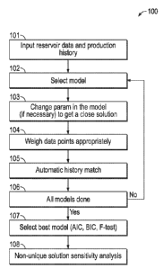
[0003] FIG. 1 is a flow diagram illustrating exemplary history matching
multi-porosity
modeling according to an embodiment of the present disclosure.
[0004] FIG. 2 is a graphical user interface providing exemplary history
matching
multi-porosity modeling data according to an embodiment of the present
disclosure.
[0005] FIG. 3A is a schematic perspective view of an exemplary dual porosity
model
according to an embodiment of the present disclosure.
[0006] FIG. 3B is a plan view of the embodiment depicted in FIG. 3A.
[0007] FIG. 4A is a schematic perspective view of an exemplary triple porosity
model
according to an embodiment of the present disclosure.
[0008] FIG. 4B is a plan view of the embodiment depicted in FIG. 4A.
CA 02932231 2016-05-31
W02015/102632 PCT/US2014/010036
[0009] FIG. 5 is a graphical user interface providing exemplary history
matching
multi-porosity modeling data according to an embodiment of the present
disclosure.
[0010] FIG. 6 is another graphical user interface providing exemplary
history
matching multi-porosity modeling data according to an embodiment of the
present
disclosure.
[0011] FIG. 7 is a graphical user interface illustrating an exemplary
model comparison
according to an embodiment of the present disclosure.
[0012] FIG. 8 is a graphical user interface illustrating another
exemplary model
comparison according to an embodiment of the present disclosure.
[0013] FIG. 9A is a graphical user interface illustrating an exemplary
comparison of
models with production data according to an embodiment of the present
disclosure.
[0014] FIG. 9B is a graphical user interface illustrating another
exemplary comparison
of models with production data according to an embodiment of the present
disclosure.
[0015] FIG. 10 is a graphical user interface illustrating an exemplary
statistical
distribution according to an embodiment of the present disclosure.
[0016] FIG. 11 is a graphical user interface illustrating another
exemplary statistical
distribution according to an embodiment of the present disclosure.
DETAILED DESCRIPTION OF DISCLOSED EMBODIMENTS
[0017] As an initial matter, it will be appreciated that the
development of an actual,
real commercial application incorporating aspects of the disclosed embodiments
can and
likely will require many implementation-specific decisions to achieve the
developer's
ultimate goal for the commercial embodiment. Such implementation-specific
decisions
may include, and likely are not limited to, compliance with system-related,
business-related, government-related and other constraints, which may vary by
specific
implementation, location and from time to time. While a developer's efforts
might be
complex and time-consuming in an absolute sense, such efforts would
nevertheless be a
routine undertaking for those of skill in this art having the benefits of this
disclosure.
[0018] It should also be understood that the embodiments disclosed and
taught herein
are susceptible to numerous and various modifications and alternative forms.
Thus, the
use of a singular term, such as, but not limited to, "a" and the like, is not
intended as
limiting of the number of items. Similarly, any relational terms, such as, but
not limited
to, "top," "bottom," "left," "right," "upper," "lower," "down," "up," "side,"
and the like,
2
CA 02932231 2016-05-31
WO 2015/102632 PCT/US2014/010036
used in the written description are for clarity in specific reference to the
drawings and are
not intended to limit the scope of the present disclosure.
[0019] In one embodiment, there can be provided a method for determining
reservoir
properties and fracture properties in oil and gas wells based on dimensionless
flow rate
using computerized modeling. A computational model generally refers to a
mathematical
model that simulates the behavior of a system, such as the production from an
oil and/or
gas well, and allows a user to analyze the behavior of the system. In an
embodiment,
modeling using a dimensionless flow rate model of a hydrocarbon well can allow
for
determining reservoir and fracture properties from data sources where daily
and/or
monthly rates are available but the flowing pressure is not available. An
example of such
a data source would be the Texas Railroad Commission public cumulative
production of
oil, water and gas for all the wells in Texas. The data from this source can
be used to
determine a flow rate, but it typically does not provide the daily pressure
data for the well,
which can be a requirement in some computational models. In an embodiment
using a
dimensionless rate solution, this or other public data can be used for
determining reservoir
and fracture properties, even though the daily pressure data may be
unavailable. This can
allow a well engineer or other user to compare wells in the same geographical
area (or
others). While embodiments of the present disclosure can use pressure
information if
available, such information is not required because both rate and pressure
exist in the
same equation. In other words, to avoid having two partial derivatives in one
equation
(making the equation underdetermined), one can be made constant. This can be
considered a significant difference between an analytical solution and a
numerical
solution. That is, in a numerical solution, both variables can change over
time; but,
during a single time step, one of them can be constant. Public production data
and
information about wells can be available from multiple sources, including, for
example,
private web services such as DrillingInfo.com, and one or more state
government's public
web service.
[0020] FIG. 1 is a flow diagram 100 illustrating exemplary history
matching multi-
porosity modeling according to an embodiment of the present disclosure. In
block 101
reservoir data and production history can be provided to a computational model
of a well.
The production history is the actual data (or relevant portions of such data)
measured at
the well while it is in operation. The full range of information can include,
for example,
pressures, temperatures, volumes of oil, water, and gas produced by the well,
and other
3
CA 02932231 2016-05-31
WO 2015/102632 PCT/US2014/010036
information gathered by the well operator. Of course, the full range of
available
production information would be known to the well operator, but may not
generally be
available to the public. Although it can be desirable to have as much
information about a
well as possible, one or more embodiments of the present disclosure can allow
accurate
modeling and determination of reservoir properties and fracture properties
using only the
oil, gas and water flow rates of the well at hand, which can be any well.
Depending on
the location of the well, operators are sometimes required to make at least
some well
information public. In the U.S., for example, public data can typically
include the
volumes of oil, water and gas produced by a particular well, such as on a
monthly or other
periodic basis.
[00211 Providing historical data to a computational model can be
performed in any
manner that allows the computational model to access the data during
operation. In one
embodiment, which is but one of many, historical data can be entered manually,
for
example, through a suitable graphical user interface ("GUI") implemented on a
computer
containing or having access to the computational model. In another embodiment,
historical data can be stored on a suitable storage medium, such as a hard
disk, CD ROM,
or flash drive that can be accessed or read by a processor, such as the
processor executing
the computational model. For example, historical data can be stored in the
form of an
Excel spreadsheet which can be accessed by the model. In still another
embodiment,
historical data can be stored on a computer system having a computer processor
separate
from the computer processor executing the computational model. For example,
the
historical data can be provided through a system configured in a client-server
architecture, where the historical data can be stored on a server computer
which can be
accessed over a computer network by the computational model that can be
running on a
client computer processor. In yet another embodiment, a computational model
can access
historical data on a remote computer, such as through the Internet or through
distributed
computing or cloud computing architectures. As an example, for a project in a
given
geographic area (which can be any geographic area), a web service, in which
the
historical data can be stored on a computer server, can be accessed by a
client computer
over the Internet. A client computer can also be the modeling computer, or it
can simply
retrieve historical data for later access by a modeling computer. Accessing
historical
data can, but need not, include filtering inputs, such as to narrow the scope
of wells from
or regarding which to obtain the production data. Filtering options or
criteria can include,
4
CA 02932231 2016-05-31
WO 2015/102632 PCT/US2014/010036
for example, latitude and longitude, public land survey, operator name, well
name, or
other information, such as well American Petroleum Institute ("API") number or
other
identifying information. Once the scope of well data has been defined, the web
service
can transfer the data to a user defined location. Once the data is made
available, the
monthly cumulative volumes for oil, water and gas that were reported to a
state, for
example, can be converted to average monthly rates in view of their
corresponding
cumulative amounts of time. An Excel spreadsheet can be useful for this
purpose. For
instance, in at least one embodiment, an application or model can read or
otherwise obtain
data from an Excel spreadsheet which, for example, can be obtained from a
comma-
separated values ("CSV") file including the data, or another source. The multi-
porosity
computational model, discussed in embodiments below, can then consume this
data and
analyze it. Other information provided in block 101 can include reservoir
data. Reservoir
data can include data about well geometry and permeability, for example. In at
least one
embodiment, which is but one of many, a GUI can be provided for allowing entry
of one
or more parameters into a model engine.
[0022] FIG. 2 is a graphical user interface providing exemplary history
matching
multi-porosity modeling data according to an embodiment of the present
disclosure. On
the right hand side of the screen in this embodiment, the GUI can allow entry
of one or
more parameters, such as, for example, matrix permeability km, man-made or
secondary
hydraulic fracture permeability kF, natural fracture permeability kf, fracture
length (or, in
some embodiments the half-length) LF, number of secondary fractures, number of
natural
fractures, and skin. In the embodiment of FIG. 2, which is but one of many,
the number
of fractures can be the length of a drainage area of the model divided by LF.
The "skin"
can be the pressure drop caused by a flow restriction in a near-wellbore
region. Of
course, it will be appreciated that this is only one embodiment, and that
additional
parameters can be added to (or omitted from) the GUI, for example, depending
on the
model used, the preferences of the system designer, or a particular
application at hand.
For example, if a computational model makes use of historical pressure
information, then
a similar entry window can be provided. The reservoir data can also be
provided in one
or more embodiments in like manners as those described with respect to the
historical
data, for example, through a spreadsheet or from suitable computer storage
media located
on the same computer executing the computational model or a remote computer
accessible over a computer network or otherwise. Similarly, in other
embodiments, the
5
CA 02932231 2016-05-31
WO 2015/102632 PCT/US2014/010036
GUI shown in FIG. 2 can be provided on the same computer as the model or on a
separate
computer disposed in communication with the model computer.
[0023] In one or more embodiments of the present disclosure, it can be
useful to hold
some of the parameters constant rather than recalculate them. This can allow a
user (e.g.,
a well engineer) to analyze how the output of the computational model can
change in
response to variations in one or more of its input parameters. Therefore, in
the GUI 200
according to the embodiment depicted in FIG. 2, check boxes 210 can be
provided to the
left of each parameter. Checking the box can provide an input to the
computational
model, for example, so that the parameter can be iteratively calculated by the
model when
executed by the system computer. If the box is unchecked, however, then this
can
provide an input to the computational model so that the model can hold the
corresponding
parameter constant while only the parameters associated with the checked boxes
can be
iteratively calculated by the computational model. Such an embodiment can be
useful in
performing sensitivity analyses, for example. It will of course be understood
that the
above-mentioned inputs can be provided in other manners as well, including in
the
reverse of the order described (i.e., unchecking a box corresponds to
iterative calculations
while checked boxes correspond to constants).
[0024] The values of one or more parameters can be displayed, such as in a
series of
windows 211 in the GUI placed in relation to each parameter. Data entry boxes
212 can
be provided, which can allow a user to enter values for each parameter. A user
initially
can provide a first set of inputs in data entry boxes 212 for the
computational model to
use as initial values for the parameters. These initial values can be
estimated based on
known or estimated values for similar wells in the area, for instance. They
can also be
chosen based on typical values or on the user's skill or experience. For
example, typical
values for porosity can be around 4 ¨ 10 percent in some formations or
locations, such as
the so-called Eagle Ford shale, for example. Details of a well design can, but
need not,
provide or suggest a maximum limit for the total number of fractures, and can
also
provide or suggest a range for other fracture properties based on other
analyses. In an
embodiment, a computational model can iteratively re-calculate values for one
or more
parameters, for example, until the model can determine a solution that matches
the
historical data. The final values of one or more parameters, such as
iteratively calculated
by the computational model, can then be displayed in one or more windows 211.
6
CA 02932231 2016-05-31
WO 2015/102632 PCT/US2014/010036
[0025]
On, for example, the left hand side of the GUI embodiment depicted in FIG. 2,
which is but one of many, a display can show a comparison of a model result
201,
indicated by the solid line, and production data 202, indicated by the series
of data points.
This can provide a visual indication of the computational model solution and
how it
performs against historical data. One or more other features can be included
in a GUI (or
plurality of GUIs), such as in the exemplary embodiment of FIG. 2. For
example, a GUI
can include controls or other inputs for one of more functions, such as for
selecting the
axes type 203, performing history matching 204, performing sensitivity
analyses 205,
weighing historic data 206, calculating a slope of the model 207, selecting
the model flow
pattern 208, separately or in combination with one or more other mechanisms,
such as for
selecting a transient or steady state analysis 209. One or more GUIs can be
implemented
as an algorithm on the same computer implementing the computational model. In
one or
more other embodiments, the GUI(s) can be implemented on a separate computer,
for
example, a computer or plurality of computers that can provide reservoir
information to a
model over a local network, over the Internet, or by way of another system for
allowing
or implementing data transfer or other communication between two or more
computers.
[0026] A transient analysis, or unsteady state analysis, can assume that
interaction
between fractures and a matrix is changing during a given flow time interval.
The pseudo
steady state analysis can assume that interaction between fractures and a
matrix is
constant during a given flow time interval.
[0027]
The initial values for the parameters supplied by a user through a GUI (e.g.,
the
GUI of FIG. 2) can be provided to a computational model of a well. Exemplary
embodiments of a computational model using a dimensionless flow rate will be
described
with respect to FIGS. 3A ¨ 4B. FIGS. 3A ¨ 4B provide schematic depictions of
geometry
that can be used according to one or more embodiments of the present
disclosure. FIG.
3A is a schematic perspective view of an exemplary dual porosity model
according to an
embodiment of the present disclosure. FIG. 3B is a plan view of the embodiment
depicted in FIG. 3A. FIG. 4A is a schematic perspective view of an exemplary
triple
porosity model according to an embodiment of the present disclosure. FIG. 4B
is a plan
view of the embodiment depicted in FIG. 4A. FIGS. 3A-4B will be described in
conjunction with one another. A well drainage area can be modeled as a
rectangular
block of subsurface matrix having a length x, width y, and a height h. The
horizontal
wellbore 301 can run through the matrix (e.g., through the middle) along
length x.
7
CA 02932231 2016-05-31
WO 2015/102632 PCT/US2014/010036
Extending outwardly along both sides of a horizontal wellbore 301 can be the
main
hydraulic fractures 302. The hydraulic fractures 302 can serve to transport
hydrocarbons
from a formation matrix to a wellbore 301. The fracture length LF can be
modeled as a
length between the main hydraulic fractures in a formation matrix, as shown in
the
figures. One-half of the fracture length, or LF/2, can be the distance from
the formation
fracture to a center of the relevant section of matrix 300. This can be seen
in the plan
view of the dual porosity geometry model shown in FIG 3B. In the dual porosity
model,
the matrix can be assigned a matrix or reservoir permeability km and each
main, or
hydraulic, fracture 302 can be assigned a permeability kF.
[0028] With continuing reference to the Figures, and specific reference to
FIGS. 4A-
4B, a triple porosity model geometry can be similar to the dual porosity model
except that
in addition to the main hydraulic fractures 402, the triple porosity model can
include
additional fractures 403 running along the length x of a formation matrix 400
to simulate
natural fractures. Fractures 403 in the triple porosity model, sometimes
referred to as
natural fractures, can be assigned a permeability kf. An exemplary geometric
arrangement of the fractures is depicted in the plan view of the geometry of
the triple
porosity model shown in FIG. 4B. The geometry of the multi-porosity models can
be
adapted to include any number of fractures required by or appropriate for a
particular
application. For example, a quad porosity model can be constructed by
extending the
model to an additional set of fractures that could be modeled, e.g., as
running along both
the length x and width y of a formation matrix, such as at the midpoint of the
matrix
height h, or at another location along height h. Such additional fractures can
be
considered to be disposed in one or more planes, such as a plane that can be
described as
the "z" plane. These fractures can also be assigned one or more permeability
designations. For convenience, in a multi-porosity model, it can be useful to
adopt the
designation k, where "i" represents an index of n number of porosities or
other variables
associated with "i" number of fractures. This notation will be adopted in
describing one
or more embodiments below, which notation those of skill in the art will
appreciate
reflects the form of a multi-porosity model.
[0029] In at least one embodiment of Applicants' present disclosure, a
linear flow of
fluid(s) through one or more of embodiments of the models described above can
be
represented by the following dimensionless linear flow, which, in Laplace
space, can be
determined by:
8
CA 02932231 2016-05-31
WO 2015/102632 PCT/US2014/010036
1 27rs
[0030] ¨ =
q(s) jr7s)COTH(-21sfype)
[0031] where q(s) is a dimensionless flow rate in Laplace space
(alternatively, q(s) can
be represented as qDL(s) or 17 wherein "DL" stands for dimensionless and the
bar over
got, indicates Laplace space), f(s) is the fracture function, and ype is the
dimensionless
reservoir half-width (rectangular geometry). The fracture function can be
given in such
an embodiment as:
3
[0032] fi (S) = (toi Fi)
[0033] where is a dimensionless interporosity parameter and co is the
dimensionless
storativity ratio. These parameters, in turn, can be represented in this
embodiment as:
Oivi
[0034] (Di = ¨
0tVt
12 ki
[0035] = ¨ ¨ Acw
LF kF
[0036] where tot is the indexed, dimensionless storativity ratio, Ac,
is the cross-
sectional area to flow (defined below) and Ai is the indexed, dimensionless
interporosity
flow. The initial conditions can be given as:
[0037] Acw = 2 h xe, where h is the reservoir thickness and xe is the
lateral length,
0i = Porosity fraction of the respective media and
[0038] Er_i = 1, Ao = 3, FN = 0, where N is the number of porosity,
i.e., dual
porosity N = 2, triple porosity N = 3, quad porosity N = 4, etc.
[0039] In a model according to this embodiment, the geometry of the well can
be
described as:
Ai I _____________________ õ
[0040] Fi= ¨ v s n+As TANH s fi+i(s)) for a pseudo steady state model
3s
and
Aif i+1(s)
[0041] 3+s f i+i(s) for a transient flow (unsteady state) model.
[0042] Returning now to FIG. 1, in block 102, a first model can be
selected, such as,
for example, a dimensionless flow triple porosity model as described above. In
such an
embodiment, which is but one of many, the number of fractures n in the model
can be
two. This model can be used to evaluate well performance according to one or
more
embodiments of the present disclosure. It will be appreciated that in at least
one
9
CA 02932231 2016-05-31
WO 2015/102632 PCT/US2014/010036
embodiment of the present disclosure, different models can be tested against
each other,
for example, to determine which model(s) provides the most accurate results
for a
particular well, which can be any well.
[0043] One or more computational models according to Applicants' disclosure
can be
computer implemented. The computational models can be created in any suitable
software programing language, such as C, C++, Java, FORTRAN, or one or more
other
languages, such as C#, F#, J#, Javascript, Python, or another language,
separately or in
combination, in whole or in part. In at least one embodiment, for example, a
computational model can be implemented in MATLAB , which can be described as a
numerical computing environment or programming language and which will be
familiar
to one or more of those with experience in the relevant art.
[0044] In
block 103, one or more parameters can be changed, for example, if
necessary or desired to obtain a close, closer or other different solution. In
one
embodiment, a chosen model can be used to determine a flow rate. The model can
be
initially run using a set of parameters with initial values, which can be
input to the model
through one or more entry boxes 212 in a GUI (see, e.g., FIG. 2). The initial
values can
be chosen by the user based on experience, or preferably, with known
information from
similar wells in the area (or another source appropriate for an application at
hand). The
initial parameters can include estimates of the permeabilities kf and kF, the
fracture length
LF and/or the cross-sectional area to flow Acw. From these values, X and co
can be
calculated, such as according to the equations described above. In block 104,
the user, if
desired, can weigh data points. Normally, relatively early production data can
tend to be
noisy and inaccurate. Therefore, relatively recent production information can
be more
helpful or accurate when forecasting the future production of a well. Block
104 can allow
a user to assign a weight to one or more data points, which can, for example,
at least help
compensate for data that may be less reliable or important than other data
(e.g., early data
versus more recent data, etc.). FIG. 5 is a graphical user interface providing
exemplary
history matching multi-porosity modeling data according to an embodiment of
the present
disclosure. FIG. 6 is another graphical user interface providing exemplary
history
matching multi-porosity modeling data according to an embodiment of the
present
disclosure. In the exemplary GUI 500 embodiment shown in FIG. 5, a group of
historical
data points can be selected in a selection box 501, which can be sized by
moving a mouse
or other input device to select only a group of points that appear to be
inconsistent with
CA 02932231 2016-05-31
WO 2015/102632 PCT/US2014/010036
the trend of other data points from a well. These points can reflect noisy or
poor
measurements, for instance, and using a pop-up box 502, for example, a well
engineer can
reduce the weight given to such points during use by a model. A model can be
instructed
to weigh one or more points according to its assigned weight, such as by way
of a weight
button 503 being activated (or deactivated, if desired).
[0045] After a model is run (or otherwise) using initial parameters and
any weighting
of data, if applicable, an automatic history match can performed in block 105.
Model
flow rates can be computed and compared to the flow rates determined from
historical
data and an error rate can be calculated. History matching can be performed by
techniques familiar to those skilled in the art, such as by nonlinear
regression. In one or
more embodiments of the present disclosure, an optimization function in MATLAB
can
be used to iteratively find a solution to the dimensionless rate model in
Laplace space as
described above. Other algorithms for performing nonlinear regression also can
be used,
as a matter of preference. Suitable nonlinear algorithms are known to those of
skill in the
art and can be implemented in, for example, C, C++, MATLAB, FORTRAN, or any
other
suitable computer language. In at least one embodiment, the iterations that
can required
to determine solutions for a computational model to determine the value of the
parameters
can be performed according to MATLAB's nonlinear regression function,
"lsqnonlin."
[0046] At the end of a regression, a history matched solution
determined in block 105
can be displayed to a user for analysis. For example, as shown on the left
hand side of the
exemplary GUI 600 of FIG. 6, an embodiment can depict a display of a history
matched
model. A historical flow rate can be shown, such as by individual data points
in a chart
601. A dimensionless model flow rate can be depicted in a curve 602.
Parameters for kf
and kF calculated by a model can be shown in a pop-up window 603. An output of
the
lsqnonlin nonlinear regression algorithm can be shown in a window as well,
such as
window 603. The actual values for the permeabilities, fracture lengths, and
other
parameters can be determined by the model through an iterative history
matching process
according to embodiments of the present disclosure. These values can then be
used by a
user to evaluate and predict the future production of a well.
[0047] With continuing reference to the Figures, and specific reference to
FIG. 1, in
block 106, a determination can be made regarding whether additional models are
to be
evaluated. This can allow a well engineer to determine whether to adjust the
parameters
and re-run a previous computational model or whether to select a different
model
11
CA 02932231 2016-05-31
WO 2015/102632 PCT/US2014/010036
altogether. At block 106, results from a history match performed in block 105
can be
compared against an acceptable error, which can be based, for example, on a
difference
between the actual and modeled production rates. The cumulative production of
fluids,
such as oil, gas, oil and water, oil and gas, or oil and water and gas, for
both an actual and
a computational model can be compared with the expectation that the error will
be less
than an amount satisfactory to the requirements set by a user, which can be
any
percentage of error.
[0048] In at least one embodiment, error can be calculated as a root-
mean-squared rate
according to the formula Error(x) = ((Qmodel(x) ¨ Qactual(x)) * weight(x)),
where x is
the value of a parameter, Qmodel(x) is the value of the parameter iteratively
calculated by
a computational model, Qactual(x) is the actual value of the parameter as
measured in, or
derived from, the historical data, and weight(x) is the influence of a data
point on the
error which affects the history match. An initial or default weight value for
all data points
can be 1 until changed by a user, although this need not be the case and each
initial
weight can be any value, whether the same as or different from one or more
other weight
values. A user can set a desired range of acceptable error as a matter of
design
preference.
[0049] In at least one embodiment, if a model flow rate falls outside a
range of
acceptable error, then the work flow can proceed back to block 102. If the
well engineer
or other user elects to re-run a then-current model, then flow can proceed to
block 103
and then block 104 where the well engineer can adjust and/or re-weigh one or
more
parameters. A computational model can then compute the history match in block
105.
This process can be repeated until a model flow rate matches a historical flow
rate to
within an acceptable error, or until a number of allowable iterations has been
reached.
The model selection can be defined by a user, for example, in MATLAB or other
source
code. At block 106, a well engineer can choose to compare one or more models,
such as
dual, triple, and/or quad porosity models, against one another to see which
model(s)
provide the best results for a subject well. Flow can proceed back to block
102, where a
different model can be chosen by a suitable entry or input to a computer, for
example, a
selection box or a command window on one or more GUI screens. The actions
described
in blocks 103-105 can be repeated for one or more models. In block 106, after
all models
which a well engineer has selected for analysis have been determined through
one or
12
CA 02932231 2016-05-31
WO 2015/102632 PCT/US2014/010036
more of the actions described with respect to blocks 103-105, flow can proceed
to block
107 for selecting a best model.
[0050] Referring still to FIG. 1, in block 107, a best model can be
selected, such as by
a user, system or combination thereof. One or more models can be compared
using one
or more statistical tools to select a model, for example, a model that most
accurately
matches the actual historical production data. Models can be compared using
the Akaike
Information Criteria, or "AIC" value. The AIC compares a model's residual sum
of
squares to the model's complexity (number of variables). A model with the
lowest AIC
value can have the highest relative probability of minimizing information loss
and the
lowest probability of overfitting or having too many parameters.
[0051] In such an embodiment, the AIC parameter can be calculated using the
following formula:
SSR 2K(K+1)
[0052] AIC = nln(¨)+ 2K +
ni n-K-1
[0053] where n is the number of data points, SSR is the sum of squared
residual, and
K is the number of parameters used in the model (i.e., Km, Kf, KF, etc.).
[0054] FIG. 7 is a graphical user interface illustrating an exemplary
model comparison
according to an embodiment of the present disclosure. FIG. 7 shows the results
of an
exemplary AIC calculation. Here, dual, triple, and quad porosity models were
compared.
It is apparent that in this example embodiment, which is but one of many, the
best model
for this particular well would be the triple-porosity model because the
probability of that
model being correct was found to be 79.7% (i.e., a higher probability than
those for the
remaining models).
[0055] In another embodiment, the models can be compared using an F-test,
which
can be calculated according to the following formula:
[0056]
SSR1- SSR2 n - p2
F= ________________________________________
SSR2 p2 ¨ pl
[0057] where n is the number of data points, SSR1 is the sum of squared
residual for
the first model, SSR2 is the sum of squared residual for the second model, p1
is the
number of parameters in the first model, and p2 is the number of parameters in
the second
model. FIG. 8 is a graphical user interface illustrating another exemplary
model
comparison according to an embodiment of the present disclosure. The results
of an
13
CA 02932231 2016-05-31
WO 2015/102632 PCT/US2014/010036
exemplary F-test, i.e., values of F from the equation above using an exemplary
set of
parameters for illustrative purposes, are shown in FIG. 8. Again, in this
example
embodiment, which is but one of many, for the particular data related to the
exemplary
well analyzed, the triple porosity is shown to be superior to either the dual
or quad
porosity models. It should be noted that the F-Test is a comparison between
two nested
models to determine if the model with more parameters yields a significantly
lower error.
Models with more parameters can result in a better fit to the actual data, but
can add
additional complexity to the task of resolving a unique solution. The P-value
is a
probability measure of the sum of squares over the degrees of freedom to
determine the
significance of one model compared to the other.
[00581 Those of skill in the art having the benefits of the present
disclosure will
appreciate that other methods of comparing models can be used. For example, in
yet
another embodiment of the present disclosure, two or more models can be
compared
using Baysian Information Criteria ("BIC"). In one or more embodiments, a well
engineer can visually display one or more model comparisons, in addition, or
as an
alternative, to one or more statistical comparisons. FIG. 9A is a graphical
user interface
illustrating an exemplary comparison of models with production data according
to an
embodiment of the present disclosure. FIG. 9B is a graphical user interface
illustrating
another exemplary comparison of models with production data according to an
embodiment of the present disclosure. FIGS. 9A, 9B show embodiments of the
present
disclosure depicting a comparison of three exemplary models (e.g., those
described herein
for illustrative purposes) with the corresponding historical production data
by way of a
graphical display. Differences in the models can be observed, for example, in
the slope of
the data as well as the accuracy of the history match. Visually inspecting the
output of
the models can be helpful in validating the overall accuracy of the output as
each model
can use the same input that might have been weighted for various reasons.
Additionally
the use of a LogLog plot can help visualize the slopes of actual and modeled
data and can
help determine when in time each flow regime occurred.
[0059] In block 108, a non-unique solution sensitivity analysis can be
performed. The
non-linear regression used in history matching in block 105 can yield non-
unique
solutions. Non-unique solutions can be problematic because different parameter
combinations can result in different solutions that satisfactorily match the
historical data,
but yield different values for the iteratively computed parameters in a model,
such as
14
CA 02932231 2016-05-31
=
WO 2015/102632
PCT/US2014/010036
matrix permeability, main hydraulic fracture permeability, porosity and so
forth. Because
different values for these parameters can result in different predictions for
an actual well
production, it can be helpful to analyze results to find unique solutions or
clear trends
between the parameters that can allow at least some confidence that the
computed
parameters match the actual formation properties. At block 108, a non-unique
solution
that can be found in a well production analysis can be the inverse
relationship between a
hydraulic fracture's length and permeability. This relationship can be
observed, for
example, in a dimensionless fracture conductivity equation and a skin factor
equation for
a hydraulic fracture. In at least one embodiment of the present disclosure,
the parameters
for a particular model can be varied within a range (which can be any range)
and the
resulting distributions can be used to determine the sensitivity of the model.
[0060] FIG. 10 is a graphical user interface illustrating an
exemplary statistical
distribution according to an embodiment of the present disclosure. FIG. 10
shows an
initial parameter distribution prepared according to an embodiment of the
present
disclosure for an exemplary set of dual, triple, and quad porosity models
using a
dimensionless flow rate determined according to a computational model as
described
herein. Uniform random sampling of one or more initial parameters can be used
to
determine aspects of the model. One or more parameters can be varied within a
range,
such as a range sufficient to include any values that are plausible based on,
for example,
area knowledge and experience. A set of initial values can be chosen based on
any
available information that a user may have regarding the corresponding
variable. For
example, a model can benefit from (i.e., by becoming more accurate or more
likely to be
accurate) a set of initial values for a variable chosen from as narrow of a
range as possible
for that value. Also, even this set can be chosen from a different
distribution, such as
Gaussian, Poisson, etc., if any a priori information is available about the
corresponding
variable. This inverse modeling problem can be non-linear and it can generate
multiple
local minima solutions. Covering the range of all possible solutions as
initial parameters
can allow a sensitivity analysis to identify most or all of the local minima,
which can
quantify an extent of any non-unique solutions. Without using a uniform random
sampling on the initial parameters it can be possible that some local minima
will never be
detected. FIG. 10 is an exemplary Bi-Plot or Matrix Plot of 2D Plots showing
relationships of each variable to all other variables in the embodiment (which
is but one
of many). Each row header in this example identifies the variable for the Y-
Axis along
CA 02932231 2016-05-31
=
WO 2015/102632
PCT/US2014/010036
the corresponding row; similarly, each column header identifies the variable
for the X-
Axis along the corresponding column. The plots along the diagonal show an
initial
histogram (e.g., a graph of a frequency distribution in which rectangles with
bases on the
horizontal axis are given widths equal to class intervals and heights equal to
corresponding frequencies) for the variable corresponding to the respective
row-column
intersections. As shown in FIG. 10 for illustrative purposes, the histograms
(and the
intervals or interlogs in the remaining graphs) can illustrate whether the
initial parameters
for a particular application were (or were not) selected with uniform
probability. In the
exemplary embodiment of FIG. 10, which is but one of many, five variables were
used,
namely, kF (main (or hydraulic) fracture permeability), kf (natural fracture
permeability),
km (reservoir (or matrix) permeability), Lf (distance between natural
fractures) and ye
(main (or hydraulic) fracture half-length), but other variables and numbers of
variables
(which can be any number) can be used in accordance with a particular
application. In
this example, two hundred initial values were selected for each variable out
of a range of
possible values for that variable, although this need not be the case and,
alternatively, any
number of initial values can be used, such as, 1, 5, 20, 50, 100, 300, 400 . .
. n values,
such as up to 5000 or more values, including any number there between
(including whole
numbers and any fractional portions of any of them). In at least one
embodiment, it can
be advantageous to use between about 100 and about 300 values for each
variable,
although this need not be the case. The data can be displayed in a log-normal
distribution, but need not be, and can alternatively be illustrated or
otherwise represented
in one or more other distributions, such as a Gaussian or other elliptical
distribution, a
circular distribution or, as another example, a Pareto distribution. In at
least one
embodiment, a model according to the disclosure can be adapted to analyze a
set of initial
values and to determine for one or more variables a best match to actual
production data.
In other words, a model can at least partially narrow a list of available
choices for the
value of one or more variables within a range of possibilities. In this
manner, a model
can identify one or more values that may be more probable than one or more
other values
to be accurate for a particular application, which can, but need not, include
identifying a
trend. Such information can be displayed to a user, for example, by way of a
GUI or
other interface, such as the one shown in FIG. 11.
[0061] FIG. 11 is a graphical user interface illustrating another
exemplary statistical
distribution according to an embodiment of the present disclosure. FIG. 11
shows a
16
CA 02932231 2016-05-31
WO 2015/102632 PCT/US2014/010036
matrix plot for the exemplary data and parameters discussed above after a
sensitivity
analysis or history match. A matrix plot can include one or more plots (e.g.,
2D images)
or subplots for identifying one or more relatively probable values for one or
more
parameters. Along a diagonal of a matrix plot can be a subplot for each
parameter, such
as a histogram which can indicate the frequency of one or more values for a
parameter.
The histogram for each parameter and/or the remaining individual subplots can
demonstrate the local minima and the probabilities for a unique solution along
with the
relationship each parameter has to other parameters. Because a triple porosity
model is
underdetermined, the solution to the inverse problem is not unique. This
problem can be
avoided, for example, by holding at least one parameter constant. With
continuing
reference to FIG. 11, subplot A, for example, can indicate to a user that, in
the example
embodiment described herein for purposes of explanation and illustration, a
most likely
value for KF can be approximately 75 (or .075 using the exemplary multiple
indicated; the
multiplier hereinafter will be ignored for simplicity). As another example,
subplot B can
indicate to a user that, in the example embodiment described herein, a most
likely value
for Kt- can be within the range of 0-50. As yet another example, subplot C can
indicate to
a user that, in the example embodiment described herein, more information can
be needed
to determine a unique solution for a value of Lf. Further, the two curves of
subplot C can
indicate to a user that, in the example embodiment described herein, there can
likely be
two solutions for a value of Lf; under such circumstances, a user can
determine which one
is best for a particular application based on, for example, other information
available to
the user about the project at hand, experience or knowledge in the field, etc.
For instance,
one or more of a plurality of unique solutions may be inapplicable in light of
certain
circumstances.
[0062] A system architecture in or with which embodiments of the present
disclosure
can be implemented can include any computer system or architecture capable of
processing or running one or more embodiments of the models disclosed herein.
For
example, one or more of the models disclosed herein can compute on an x86, x64
or
ARM based processor running on one of many available operating systems (e.g.,
MAC,
WINDOWS, ANDROID, LINUX, etc.), and can do so regardless of whether a computer
system available to a user includes a graphics processor for visualization.
For example, in
the event available computer hardware does not include a graphics processor, a
command
console (e.g., MSDOS, LINUX, etc.) can be used to setup, run and/or
export/view one or
17
CA 02932231 2016-05-31
WO 2015/102632 PCT/US2014/010036
more model outputs, such as by way of texts, characters, strings or other
applicable
designations.
[0063] A computer implemented method can include selecting a first flow rate
model
for a well, the first flow rate model having at least one input parameter,
providing data to
the first flow rate model, such as reservoir data and production history data,
computing
one or more solutions to the first flow rate model, which can include using an
initial value
for a input parameter, comparing a solution to production history data,
adjusting an input
parameter, computing a solution to the first flow rate model using one or more
adjusted
input parameters, selecting a second flow rate model for a well, the second
flow rate
model having at least one input parameter, providing reservoir data to the
second flow
rate model, providing production history data to the second flow rate model,
computing
one or more solutions to the second flow rate model, which can including using
one or
more input parameters, comparing a solution to production history data,
adjusting an
input parameter, computing a solution to the second flow rate model using one
or more
adjusted input parameters, comparing a solution from the first model with a
solution from
the second model, and determining which model most accurately tracks the
production
history data.
[0064] A first flow rate model can include a multi-porosity
dimensionless flow rate
model, which can include a dimensionless flow rate model of the form
2 gs
[0065]¨ = ¨COTH(-21FsfrOyDe).
q(s) s f (s)
[0066] An input parameter can represent reservoir data and can include one or
more
values representing one or more of formation matrix permeability, hydraulic
fracture
permeability, fracture length, and a combination thereof. A method can include
determining whether a model solution that most accurately tracks the
production history
is unique, which can include varying an input parameter over a range of values
and
determining a plurality of model solutions. Production history data can
include data
representing a volume of oil, water, and/or gas produced by a well over a time
period. A
method can include iteratively adjusting an input parameter and computing a
solution to a
flow rate model until a solution is within an error criteria, and can include
statistically
comparing a solution from a first model with a solution from a second model,
which can
include determining a value based on one or more of the Akaike information
criteria, the
F-Value, the Baysian information criteria, and a combination thereof.
18
CA 02932231 2016-05-31
WO 2015/102632 PCT/US2014/010036
[0067] A computer readable medium can have instructions stored thereon that,
when
executed by a processor, can cause the processor to perform a method that can
include
selecting a first flow rate model for a well, the first flow rate model having
at least one
input parameter, providing data to the first flow rate model, such as
reservoir data and
production history data, computing one or more solutions to the first flow
rate model,
which can include using an initial value for a input parameter, comparing a
solution to
production history data, adjusting an input parameter, computing a solution to
the first
flow rate model using one or more adjusted input parameters, selecting a
second flow rate
model for a well, the second flow rate model having at least one input
parameter,
providing reservoir data to the second flow rate model, providing production
history data
to the second flow rate model, computing one or more solutions to the second
flow rate
model, which can including using one or more input parameters, comparing a
solution to
production history data, adjusting an input parameter, computing a solution to
the second
flow rate model using one or more adjusted input parameters, comparing a
solution from
the first model with a solution from the second model, and determining which
model
most accurately tracks the production history data.
[0068] In a computer readable medium can have instructions stored
thereon, a first
flow rate model can include a multi-porosity dimensionless flow rate model,
which can
include a dimensionless flow rate model of the form
27rs
[0069] ¨ = ¨COTH(-2.9VDe).
q(s) (s)
[0070] An input parameter can represent reservoir data and can include one or
more
values representing one or more of formation matrix permeability, hydraulic
fracture
permeability, fracture length, and a combination thereof. A method can include
determining whether a model solution that most accurately tracks the
production history
is unique, which can include varying an input parameter over a range of values
and
determining a plurality of model solutions. Production history data can
include data
representing a volume of oil, water, and/or gas produced by a well over a time
period. A
method can include iteratively adjusting an input parameter and computing a
solution to a
flow rate model until a solution is within an error criteria, and can include
statistically
comparing a solution from a first model with a solution from a second model,
which can
include determining a value based on one or more of the Akaike information
criteria, the
F-Value, the Baysian information criteria, and a combination thereof.
19
CA 02932231 2016-05-31
WO 2015/102632 PCT/US2014/010036
[0071] While the disclosed embodiments have been described with reference to
one or
more particular implementations, those skilled in the art will recognize that
many changes
may be made thereto without departing from the spirit and scope of the
description.
Accordingly, each of these embodiments and obvious variations thereof is
contemplated
as falling within the spirit and scope of the claimed invention, which is set
forth in the
following claims.