Note: Descriptions are shown in the official language in which they were submitted.
CA 02932782 2016-06-10
56002306-2CA
- 1 -
ORIENTATION MODEL FOR INERTIAL DEVICES
TECHNICAL FIELD
The present disclosure relates to methods and systems for determining the
orientation of
a moving object in three-dimensional space, such as those found in inertial
navigation systems,
inertial measurement units, and magnetic angular rate and gravity sensor
arrays.
BACKGROUND OF THE ART
Orientation estimation of a moving object in three-dimensional space is a
challenging
problem, which has vast applications in gaming, avionics, wearable devices,
etc. The
orientation estimation can be performed either online using a microcontroller
on the device, or
offline using a separate computer, depending on the application. While offline
approaches can
support complex calculations, online approaches have different requirements,
such as real-time
calculations and low power consumption. Utilizing low-cost and low-power
microcontrollers for
real-time applications is not compatible with orientation estimation
techniques that involve
intensive arithmetic computations.
Conventional orientation estimation methods are based on either using direct
Euler angle
representations or the quaternion representation. A quaternion is a four-
dimensional complex
number that can be used to represent the orientation of a rigid body or
coordinate frame in
three-dimensional space. The quaternion representation avoids trigonometric
matrix
calculations, and thus, is more efficient computationally compared to the
Euler angle
transformations. Furthermore, Euler angle representations suffer from
singularity conditions,
which is not the case with the quaternion model.
Some solutions exist which make use of the quaternion representation for
orientation
estimation, namely Kalman-based methods. Although accurate, these methods are
not
computationally-efficient for low-power embedded applications. In fact, Kalman
filters involve
matrix inversions, covariance matrix calculations, etc., which makes them
inefficient to meet the
low power and real-time performance constraints imposed by some applications.
Another solution, known as the Madgwick orientation filter, is a
computationally-efficient
method, which makes use of the quaternion representation and is suitable for
low-power real-
time applications. However, there is a need for improved overall accuracy of
the filter, without
3 0 increasing computational costs.
CA 02932782 2016-06-10
56002306-2CA
- 2 -
SUMMARY
There is described a computationally efficient quaternion-based orientation
estimation
model for a moving object using a specialized gradient descent correction
step.
In accordance with a first broad aspect, there is provided a computer-
implemented
method for estimating an orientation of a moving object in three-dimensional
space. The
method comprises obtaining filtered and calibrated angular velocity readings
of the object;
computing a first correction vector by directing a quaternion orientation
estimate at time t-1
towards the angular velocity readings found at time t to generate a quaternion
orientation
estimate of the angular velocity readings at time t; obtaining filtered and
calibrated proper
acceleration readings of the object; computing a second correction vector by
directing the
quaternion orientation estimate of the angular velocity readings at time t
towards the proper
acceleration readings found at time t; and using the second correction vector
as a
measurement error for estimating the orientation of the moving object at time
t.
In some embodiments, the method further comprises obtaining filtered and
calibrated
heading angle readings of the object, and wherein computing the second
correction vector
comprises directing the quaternion orientation estimate of the angular
velocity readings at time t
towards the proper acceleration readings and the heading angle readings found
at time t.
In some embodiments, the method further comprises detecting a temporary
disturbance
in the proper acceleration readings at time t, and adjusting the second
correction vector at time
t to account for the temporary disturbance. In some embodiments, adjusting the
second
correction vector at time t comprises applying at least one confidence weight
to the proper
acceleration readings, and adjusting the confidence weight at time t when the
temporary
disturbance is detected.
In some embodiments, the method further comprises detecting a temporary
disturbance
in at least one of the proper acceleration readings and the heading angle
readings at time t, and
adjusting the second correction vector at time t to account for the temporary
disturbance.
In some embodiments, the method further comprises determining a zero-bias
drift in the
angular velocity readings for stationary positions of the object by computing
a mean value of the
angular velocity readings, and correcting for the zero-bias drift.
In some embodiments, the method further comprises determining a zero-bias
drift in the
angular velocity readings for stationary or non-stationary positions of the
object using the
quaternion orientation estimate at time t-1, and correcting for the zero-bias
drift.
CA 02932782 2016-06-10
56002306-2CA
- 3 -
In some embodiments, the first correction vector and the second correction
vector are
both quaternions, computing the first correction vector comprises numerically
integrating a
quaternion derivative which is found using the proper angular velocity
readings, and computing
the second quaternion comprises computing a gradient descent.
In some embodiments, the method is implemented by an inertial measurement unit
(IMU)
sensor array. In some embodiments, the method is implemented by a Magnetic
Angular Rate
and Gravity (MARG) sensor array.
In accordance with another broad aspect, there is provided a system for
estimating an
orientation of a moving object in three-dimensional space. The system
comprises a processing
unit and a non-transitory memory communicatively coupled to the processing
unit and
comprising computer-readable program instructions. The instructions are
executable by the
processor for obtaining filtered and calibrated angular velocity readings of
the object; computing
a first correction vector by directing a quaternion orientation estimate at
time t-1 towards the
angular velocity readings found at time t to generate a quaternion orientation
estimate of the
angular velocity readings at time t; obtaining filtered and calibrated proper
acceleration readings
of the object; computing a second correction vector by directing the
quaternion orientation
estimate of the angular velocity readings at time t towards the proper
acceleration readings
found at time t; and using the second correction vector as a measurement error
for estimating
the orientation of the moving object at time t.
In some embodiments, the memory and processing unit are provided on a single
integrated circuit as part of a microcontroller. In some embodiments, the
system is embedded
on the object.
In some embodiments, the program instructions are further executable by the
processing
unit for obtaining filtered and calibrated heading angle readings of the
object, and wherein
computing the second correction vector comprises directing the quaternion
orientation estimate
of the angular velocity readings at time t towards the proper acceleration
readings and the
heading angle readings found at time t.
In some embodiments, the program instructions are further executable by the
processing
unit for detecting a temporary disturbance in the proper acceleration readings
at time t, and
3 0 adjusting the second correction vector at time t to account for the
temporary disturbance.
In some embodiments, adjusting the second correction vector at time t
comprises
applying at least one confidence weight to the proper acceleration readings,
and adjusting the
confidence weight at time t when the temporary disturbance is detected.
CA 02932782 2016-06-10
56002306-2CA
- 4 -
In some embodiments, the program instructions are further executable by the
processing
unit for detecting a temporary disturbance in at least one of the proper
acceleration readings
and the heading angle readings at time t, and adjusting the second correction
vector at time t to
account for the temporary disturbance.
In some embodiments, the program instructions are further executable by the
processing
unit for determining a zero-bias drift in the angular velocity readings for
stationary positions of
the object by computing a mean value of the angular velocity readings, and
correcting for the
zero-bias drift.
In some embodiments, the program instructions are further executable by the
processing
unit for determining a zero-bias drift in the angular velocity readings for
stationary or non-
stationary positions of the object using the quaternion orientation estimate
at time t-1, and
correcting for the zero-bias drift.
In some embodiments, the first correction vector and the second correction
vector are
both quaternions, computing the first correction vector comprises numerically
integrating a
quaternion derivative which is found using the proper angular velocity
readings, and computing
the second quaternion comprises computing a gradient descent.
In some embodiments, obtaining the various readings for use in the method
and/or by the
system comprises measuring such data using appropriate measurement devices,
such as
gyroscopes, accelerometers, and/or magnetometers, and correcting (i.e.
filtering and
calibrating) such data accordingly. In some embodiments, obtaining the
readings comprises
receipt of such data from another source which has obtained the readings and
corrected them if
required. In some embodiments, the source from which the readings are received
is local while
in other embodiments, the source is remote.
The methods and systems described herein may be used for online and/or offline
applications.
The following notations and definitions will be used throughout the present
disclosure.
Definition 1: The Euler angles are denoted in the reference (Earth) frame with
North, East
and Up vectors as follows:
Yaw rotation around z-axis (Up) in the reference frame.
3 0 Pitch 0: rotation around y-axis (East) in the reference frame.
Roll (I): rotation around x-axis (North) in the reference frame.
CA 02932782 2016-06-10
56002306-2CA
- 5 -
The Euler angles are defined in the so-called aerospace sequence, where
rotation
around the z-axis (Yaw) takes place first, which is then followed by Pitch and
Roll, respectively.
The analysis is also applicable to other rotation sequences and Earth frames
as well.
Definition 2: The IMU/MARG sensor frame (ridged body) uses 2, ji,2 as the
principal axes,
which correspond to the sensor readings.
Definition 3: The unit-length quaternion CI
-.r,t = [qr,t,1 qr,t,2 qr,t,3 qr,t,4], where 11c1r.t11 =
Vc1r,t,i2 + qr,t,22
+ a .r,t,32 qr,t,42 = 1, represents the actual (reference) orientation of
the sensor
frame relative to the earth frame at time t. The conjugate of cir ,t will swap
the relative frames
and is defined as:
¨ [qr,t,1 qr,t,2 ¨ qr,t,3 ¨ qr,t,4 =
I
Definition 4: The quaternion estimation at time t is denoted as:
ciest,t ¨ [qest,t,1 qest,t,2 qest,t,3 qest,t,4],
which is found by the orientation filter. The error in orientation estimation
at time t is
represented as:
eq,t = ciest,, ¨ ckt = req,t,1 eq,t,2 eq,t,3 eq,t,41=
That is to say:
eq,c,j = clest,t,i ¨ cir,t,i, where j c [1,2,3,41.
Definition 5: The Hamilton product of the two quaternions cla = [cla,1 qa,2
qa,3 q4],
qb = [q b,1 qb,2 qb,3 qb,4], results in another quaternion, which is given by:
a., qb,, -qa.2qb,2-q.,-.3cib,3-qa,4qb.4
qaocib _ cialcib.2 13
+qa,2%,i+qa3q,4-qa,4%,3
(I -T
{
cla,lcib,3¨qa,2c1b,4+qa,3qb,i+qa,4c1b,2 .
qa,iqb,4+qa,2c1b,3¨qa,3c1b,2-1-qa,49b,i_
It is notable that qaeqb # qb0cia.
Definition 6: The current calibrated accelerometer, magnetometer, and
gyroscope
readings in the sensor frame at time t are denoted as Sat = (an, as, an), sm,t
-.,-- (m2, m, m2), and
Sg,t = (gn, gy, gn), respectively. The current accelerometer/magnetometer
(Acc/Mag) readings at
time t are together represented as Samt = tSa,t,SmAl. Note that regarding the
IMU filter, since
there is no magnetometer, Samt = Sat.
CA 02932782 2016-06-10
56002306-2CA
- 6 -
The sensors are considered to have passed the initial necessary low-pass
filters and to
be time synchronized. The calibrated accelerometer/magnetometer data S, S,õ,,
are also
considered to have passed a normalization step to represent unit-length
readings, i.e., IlSa,t11 =
11Sm,t11= 1. We also denote the norm of Acc/Mag readings pre-normalization as
1%,t11 and
0m,t11. These norm values are used in detecting temporary disturbances in
calibrated Acc/Mag
readings, while the normalized calibrated readings Sat, Sint are used in the
normal filter
operation mode.
Definition 7: The error in current calibrated accelerometer, magnetometer and
gyroscope
readings Sat, Smt, Sg,, are denoted as (ax' eay, eaz), (emx, emy, emz) and
(e'gx, gy, e gz) , respectively.
BRIEF DESCRIPTION OF THE DRAWINGS
Further features and advantages of the present invention will become apparent
from the
following detailed description, taken in combination with the appended
drawings, in which:
Fig. 1 is a flowchart of an exemplary method for estimating an orientation of
a moving
object in three-dimensional space;
Fig. 2 is a block diagram of an exemplary orientation model for obtaining a
correction
vector q,iv,t;
Fig. 3 is a block diagram of an exemplary implementation of the orientation
model of
figure 2 for an IMU filter;
Fig. 4 is a block diagram of an exemplary implementation of the orientation
model of
figure 2 for a MARG filter;
Fig. 5 is an exemplary graph of the reference pitch angles showing variable
angular
velocities;
Fig. 6 is an exemplary graph tracking the offset drift in pitch using two
filters featuring a
45 second step-response time; and
Fig. 7 is an exemplary system for implementing the method of Fig. 1.
It will be noted that throughout the appended drawings, like features are
identified by like
reference numerals.
CA 02932782 2016-06-10
56002306-2CA
- 7 -
DETAILED DESCRIPTION
Figure 1 is an exemplary flowchart of a computer-implemented method for
estimating an
orientation of a moving object in three-dimensional space. At least two types
of readings are
obtained from the moving object, namely angular velocity readings and proper
acceleration
readings, as per 102, 104. The proper acceleration may be obtained using a
device such as an
accelerometer. The angular velocity may be obtained using a device such as a
gyroscope. Any
other measuring device capable of obtaining this data may also be used. In
some
embodiments, a third type of readings are also obtained. They are heading
angle readings of
the object, as illustrated in optional step 105, and they may be used for
certain applications or
simply to provide a gain in performance, as will be explained in more detail
below. The heading
angle may be obtained using a device such as a magnetometer.
As per 106, the angular velocity readings are used to compute a first
correction vector.
The first correction vector takes the form of a quaternion orientation
estimate based on the
angular velocity readings of the object at time t. It is obtained by directing
a quaternion
orientation estimate at time t-1 towards the angular velocity readings found
at time t. The first
correction vector is then used in conjunction with the proper acceleration
readings to compute a
second correction vector, as per 108. The second correction vector is a result
of directing the
quaternion orientation estimate of the angular velocity readings at time t
towards the proper
acceleration readings found at time t. If the acceleration readings are
improper due to the
presence of a temporary high external force, the second correction vector may
be adjusted with
a confidence weight. As per 110, the second correction vector may then be used
as a
measurement error for estimating the orientation of the moving object at time
t.
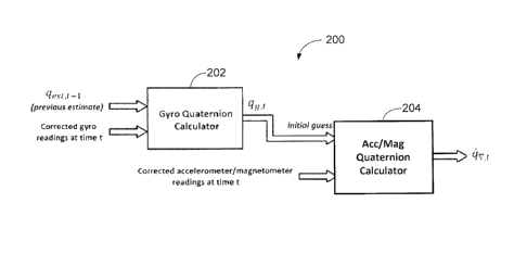
Figure 2 is an exemplary illustration of an orientation model 200 for
obtaining the second
correction vector, labeled as q. A gyro quaternion calculator 202 receives as
input an initial
guess at time t=0, which becomes a previous estimate a
after a first iteration of the process.
Corrected angular velocity readings are also received. These readings are said
to be corrected
in that they have been filtered, calibrated, and normalized where necessary
for further
processing. The gyro quaternion calculator 202 computes the first correction
vector, labeled as
qfl,t, which is a quaternion orientation estimate of the angular velocity at
time t. The output of
the gyro quaternion calculator 202 may then be used as one of the inputs to an
Acc/Mag
quaternion calculator 204, as its initial guess/qest,t-1 input. The other
input of the Acc/Mag
quaternion calculator 204 is the corrected proper acceleration readings and in
some
embodiments, heading angle readings. The Acc/Mag quaternion calculator 204
computes qt,
which is the second correction vector. The Acc/Mag quaternion calculator 204
is responsible for
rejecting the effect of temporary disturbance in calibrated Acc/Mag readings
as well.
CA 02932782 2016-06-10
56002306-2CA
- 8 -
In some embodiments, the orientation model 200 of figure 2 is applied as an
orientation
filter for Inertial Measurement Unit (IMU) sensor arrays. One such example is
illustrated in
figure 3. In some embodiments, the orientation model 200 of figure 2 is
applied as an
orientation filter for Magnetic Angular Rate and Gravity (MARG) sensor arrays.
One such
example is illustrated in figure 4. These two embodiments will be described
concurrently with
regards to certain aspects of the functionality of the orientation filters
300, 400.
The IMU and MARG sensor readings are assumed to have initially passed the
necessary
calibration, filtering, and normalization techniques, which are represented by
the initial
calibration and filtering modules 302a, 302b, 402a, 402b. For instance, low-
pass or high-pass
filters might be used to remove the undesirable frequencies from sensor
readings depending on
the application. Calibration techniques may aim to remove the potential offset
and gain from
sensor readings. Generally, for a 3-axis raw sensor reading X3õ1, the
following calibration may
be performed:
Xcalib = G3x3X C3õ, (1)
where G3x3 is the gain matrix and C3x1 is the offset. For instance, regarding
accelerometers, the values of G3x3 and C3x1 can be found using six stationary
positions and a
linear least-squares fit solution. Furthermore, regarding magnetometers, a
least-squares
ellipsoid fit may be used to find G3x3 and C3õ and remove the magnetic
distortion, including
hard iron and soft iron effects along with sensor axes misalignments . Note
that regarding
accelerometer and magnetometer readings, a normalization step may take place
post-
calibration to represent unit-length vectors.
The delay elements (Z-1) 304, 404 may be registers that capture the previous
estimate
qest,t-i and use it as a feedback input to the systems 300, 400. Note that
initially at time t = to,
we can reset the quaternion estimate qest,to to qest,,, = [1 0 0 0], which
indicates that all Euler
angles are initially zero.
The gyro quaternion correctors 306, 406 directly predict the quaternion
derivative qa,t
using the information from gyros Sfl,, as well as the previous estimate
qõ,,t_l as follows:
4,g,t ¨ chistit-10[0 gid= (2)
After obtaining gg,t in Eq. (2), we can find an initial estimate for
quaternion orientation at
3 0 time t using the integrators 308, 408 as follows:
(49,t == + tLt, (3)
CA 02932782 2016-06-10
56002306-2CA
- 9 -
where At is the sampling period and 4fl,, is given by Eq. (2).
The Acc/Mag quaternion correctors 310, 410 predict a correction vector that
pushes the
initial guess qinit, where qinit = q9,t, towards a unit-length quaternion q
that ideally matches the
Acc/Mag readings Sam,. In the case of the IMU filter 300, the block 310 is
called the
accelerometer quaternion corrector, since magnetometers are not used.
Quaternion correctors
310, 410 will generate the following output:
4v,t at(qtnit (0= at(q,g,t (4)
where a, > 0 is an arbitrary gain depending on how fast the estimator is
pushing its initial
guess qinit towards q. If at = 1, then by removing the correction vector cv,,
from the initial guess
qii we would reach the reference quaternion q:
q qinit ¨ 47,t = q9,t qv,t= (5)
If the initial guess qtnt, is close to q, the estimate c
can be found with good precision
using optimization methods, such as Newton-Raphson and Quasi-Newton solutions.
However,
such methods come with a high computational cost, which is not desirable in
low-power
embedded applications. A computationally-efficient single-step gradient
descent solution may
be used to find the correction vector
Note that one can use more iterations within the
gradient descent step, if needed. The proposed gradient descent solution makes
use of the
initial guess qinit = qq,t, which is given by Eq. (3).
The gradient descent step delivers the following correction quaternion:
(1v,t = F (clap Sam,t), (6)
where VP is the gradient of the function F, which is given below:
F(qg,t, Sõ,,t) = 12Fg(qg,t,Sõ,,,t)TF,q(q9,t, Sam,t)= (7)
The function Fg(gy,t,S) is arbitrarily chosen to represent the mismatch
between the
Acc/Mag readings Sam,t and the initial guess qfl,t = 2,
a a al For the IMU filter 300, we can
µ
use the following mismatch function:
2 (q2q4 q1q3) a2Fq(qg,t,S,,t) = qa*
,t0909,g,t Sa,ty=[0 0 0 2 (ch. q3q4) cti)
(8)
1 ¨ 2(q22 q32)
"2-3x1
CA 02932782 2016-06-10
56002306-2CA
- 10 -
where g -= [0 0 0 1] is a quaternion representing the reference gravity vector
in the Earth
frame.
The gradient in Eq. (6) is then computed as follows:
= = Ji...g(q9,t)T Fg(qg,t,Sarg,t), (9)
where JF3(qfl,t) is the Jacobian of Ffl at q = qmt. Considering Fg in Eq. (8),
we get:
-3F9,1 399,3 a,1
3q2 3q3 3,14 2q4 ¨291 2q2-
a F9,2 a F9,2 aF9,2 a F,g,2
Fg (C g ,t) = 3q1 3q2 3q3 3q4 2q2 2q1 2q4 2q3 , (10)
0 _.
399,3 399,3 3123,3 399,3 - 0 ¨4'72 ¨4q3 3x4
- aql 0q2 3q3 3(14 -
where F9,1 (j = 1,2,3), is the ith row of Fg.
The final adders 312, 412 remove the correction vector av,t multiplied by a
gain, i.e., )6 At,
where At is the sampling period, from the gyros' estimate found at time t,
i.e., qa,t in Eq. (3):
gest,t = Cig,t ¨ (flAt)c)v,t, (11)
The tunable gain )3 can be set adaptively based on sensor characteristics and
the
presence of disturbance in sensor readings to achieve optimal accuracy. We
might also set a
default optimal value for )3, where initially a higher gain is chosen to
provide convergence.
The normalizers 314, 414 normalize the estimate 0õt,, in Eq. (11) to deliver
the new unit-
length quaternion estimate gest t = qest,t
'
The zero-bias drift effect of gyroscopes can be compensated by detecting
stationary
positions and finding the mean value of the gyro readings. However, such
methods are not
capable of removing the bias drift, as the device is moving. For that purpose,
a gyro zero-bias
drift estimator 416 may be used for the MARG filter 400 to predict the zero-
bias drift in
gyroscope readings over time Sb,t.
The zero-bias value for gyros can be represented by the DC component of the
gyros'
quaternion error at time t, i.e., (2a
µe*st,t-106,3, and it can be found using the following
integrator:
Sh,t =Et(2cle*st,t-lakt)At, (12)
CA 02932782 2016-06-10
56002306-2CA
- 11 -
where is another filter gain representing the response time in
tracking the zero-bias
drift. Since the zero-bias drift phenomena takes effect slowly over time, we
can set to a small
value. The bias values Sb,t are initially subtracted from the gyro readings
.Sfl,t, and later, the
corrected readings .59,t. ¨ Sb,t are fed through the gyro quaternion estimator
406. Note that we
may initially set = 0, until gyros' estimate converges to the Acc/Mag
readings, and then we
switch to the optimal values of f3 and
The Acc/Mag quaternion corrector 410 makes use of the information from the
initial
guess tig,, (current gyro estimate) in its gradient descent initialization to
compute the correction
vector qv,t. This results in an overall performance improvement of the filter
in tracking the zero-
bias drift in gyro readings, since 4v,, directly represents the mismatch
between the current gyro
estimate and the current Acc/Mag readings.
Presented below is one possible way to realize the calculations required for
the proposed
IMU filter structure 300 in figure 3. The following steps can be taken to
realize the IMU filter 300
starting from the initial quaternion qõ,,0 = [1 0 0 0] at t = 0.
Step 1 (Finds (A) in Fig. 3): Calculate the gyro estimate q.9,, =
[q1,q2,q3,q4] using Eq. (2)
and Eq. (3):
qfl,t = + gest,t-10[0 92 99
92]. (13)
Step 2: Build the mismatch function Fa(qg,t,S) as follows:
2(q2q4 q1q3)
9=10 0 0 1]
(gg,t, Sat) = (19*,t0g0qmt Sa,t ___________ > 2 (ch 92 + q3q4)
(14)
_1 ¨ 2(q22 + q32) ¨ a2 3xi
Step 3: Find the Jacobian of Fa at q = q9 = [q1,q2,q3, q41:
¨2q2 2q4 ¨2q1 2q2
Jpa,= 2q2 2q1 2q4 2q3 (15)
0 ¨4q2 4q3 0 13x4
Step 4 (Finds (B) in Fig. 3): Use the mismatch function Fa(q.g,t,S) from Step
2 and its
Jacobian in Step 3 to find the quaternion correction as follows:
= V F(qg,t, Sa,t) = JpaT Fa. (16)
Step 5 (Finds (C) in Fig. 3): Find the new estimate:
CA 02932782 2016-06-10
56002306-2CA
- 12 -
qest,t = (1g,t )8IAt(4\7,t), (17)
where 13 may be set based on the sensor error characteristics to achieve
maximum
accuracy. We can use multiple modes to set different values of
Namely, one can choose a
higher gain for /3, i.e., ,6) = f3fast, when a high mismatch is observed
between the sensor
readings, e.g., when I IFal I or maxi(Fc, J1) exceeds a certain threshold,
where Fa,' is the ith row of
Fa. Using such an approach, the gyro readings are pushed faster towards
accelerometer
readings, when a high mismatch is observed between the sensor readings, e.g.,
in the
beginning during convergence. As the estimates get closer to each other, i.e.,
Pall and
maxi(F,01) become low enough, we will switch back to the lower and optimal
value of /3 to
observe a smoother response.
When a major external force is observed by accelerometers, e.g., Pa,t1I 1 01
Ilga,t11
1, we can also temporarily set a lower gain for /3, even )6' = 0 to completely
reject the effect of
the observed temporary external force.
Step 6 (Finds (D) in Fig. 3): Normalize a
,est,t, i.e., -4est,t to
deliver a unit length
quaternion estimate
A sample realization of the proposed MARG filter 400 in Fig. 4 is provided
below.
Step 1 (Finds (A) in Fig. 4): Remove the gyros' zero-bias drift Sb,t from gyro
readings Sfl,,,
i.e.,
¨ Sb,t,2, .037/ ¨ Sb,t,3, .02 ¨ Sb,t,4,
(18)
where initially at t = 0, the bias values Sb,t are all zero, i.e.,
(19)
Furthermore, at t = 0, we have: qõt,o = [1 0 0 0].
Step 2 (Finds (B) in Fig. 4): Use
from from Step 1 to find the gyros' quaternion
estimate at time t, i.e., qmt = [q, q2 q3 q4], as follows:
At
qest,t_i + ¨2 qõt,t_i0[0 g 21 (20)
Step 3: Build an appropriate mismatch function P(q9,,,Sam,t) between the
initial gyro
estimate q a,t from Step 2, and the Acc/Mag readings Samt.
CA 02932782 2016-06-10
56002306-2CA
- 13 -
k tF,
P(qinit,Sam,t), 6xi (21)
km,Fm1 '
where Fa (Fm) is the mismatch between qfl,, and the accelerometer
(magnetometer)
readings Sa,, (S,,,,t), while ka,t, km,t are confidence weights. We choose to
set qinit qfl,, in Eq.
(21). Consequently, the function Fa in Eq. (21) is found by Eq. (14), and Fm,
which is the
mismatch between qsõ and the magnetometer readings Smt, can be defined as
follows:
Fm(qa,t,Smt) = qfl* ,t0E0q9,, ¨ Sm,t
¨ q32 ¨ 42) + 2bz(q2q4 ¨ q1q3) ¨ mf
E= (1
J0 bx 0 bz]
_______________________________________________________ >= 2bx(q2q3 Cl1C14)
2bz(q1C12 Cl3C14) m , (22)
2bx(q1q3 + q2q4)+ 2b(0.5 ¨ q22 ¨ q32) m
3xi
where qa,, = [q1 q2 q3 q4], and E = [0 I), 0 bz] is the earth's magnetic field
in the reference
Earth frame defined by Definition 1. We also have:
b,= cos(6), and I), = ¨sin(8), (23)
where ¨90 5_ S 5_ 90 is the fixed dip angle depending on the geographic
location on
earth. The values of bx,bz can be found using several methods, e.g., directly
from the
geographic location information, or by de-rotation of magnetometer readings
back to the
horizontal plane. Alternatively, we can find these values using the inner
product of
accelerometer and magnetometer readings. To do this more efficiently, a one-
time solution
would be to initially put the device in a stationary position for ¨1-2 seconds
and find the mean
values of the calibrated and normalized accelerometer and magnetometer
readings S and
Sm,t as St, mean and 5m mean'
Next, we find the dip angle information by calculating the inner product of
the mean
values of the Acc/Mag readings:
bz = ¨sin(8) = Sa mean,m mean); b = \It ¨ 6,2.
The above values of bx,b, are initially stored in memory and will then be used
as
constant parameters for the orientation filter 400.
The function Fm in Eq. (22), which represents the mismatch between the gyro
estimate
qv and magnetometer readings, might be defined in a different way depending on
the type of
information we receive from the corrected magnetometers. For example, one
might utilize an
intensive calibration and tilt-compensation algorithm for magnetometers, and
directly find the
CA 02932782 2016-06-10
56002306-2CA
- 14 -
yaw angle components cos(V)),sin(0), in the xy horizontal plane. These yaw
angle components
might also be provided by another external source, e.g., a camera. Under such
conditions, the
mismatch function Fm in Eq. (22) can be simplified to:
2(0.5 ¨ (132 _ q42) _
cos(Vi)
Fm(q9,,,Smõ) = 2(q2q3 q1c/4) sin(i) , (24)
0 3x1
where q9,,= [q, q2 q3 q4], and the last row of Fm refers to the z-axis
component in the xy
horizontal plane, which is zero.
The confidence weights k,,,,, km.,, will determine the amount of confidence we
put in
accelerometer and magnetometer readings at time t, respectively. This is
particularly helpful in
rejecting a temporary disturbance in Acc/Mag readings after initial
calibration.
For simplicity, we can choose Boolean values for k,,,,, as follows.
Whenever a major
disturbance or external force is observed by magnetometer (accelerometer)
readings at some
time t = t1, we can temporarily set km, -= 0 (kõ,, = 0), at t = t,. When the
magnetometer
(accelerometer) disturbance is gone, we switch back to the default value of
km, = 1 = 1).
Disturbance can simply be detected when the magnitude of the calibrated
accelerometer
or magnetometer readings pre-normalization, i.e., 11-^Cci,t11 or Vin,t11,
exceeds its pre-defined
disturbance-free upper/lower bound. The reason for this is that the gravity
vector and the
Earth's magnetic field have constant magnitude values for a certain geographic
location, i.e.,
ga,t11
1g, and lIgm,11 =-z5 Bo, where Bo is the expected magnetic field intensity
post-calibration.
The disturbance-free upper/lower bounds for accelerometers and magnetometers
are defined
2 0 based on the initial calibration procedure.
In order to detect temporary disturbance on magnetometer data more accurately,
we
should additionally check the inner product of accelerometer and magnetometer
vectors
(5õ,t,Sm,t), and if the result exceeds its pre-defined disturbance-free
upper/lower bound, we can
set kmõ = 0. The reason for this condition is that the dip angle 6 between the
disturbance-free
calibrated and normalized accelerometer and magnetometer vectors is fixed for
a specific
geographic location, i.e., (Sõ,,,S,õõ)
¨sin(S). If the magnetic field is disturbance-free, i.e.,
An,t11 Bo and (So,t,Sõ,,t)
¨sin(6), then we set the default value of km, = 1 for normal filter
operation.
In summary, the confidence weights k,,,,, km, in Eq. (21) can be set using the
following
3 0 conditions:
CA 02932782 2016-06-10
56002306-2CA
- 15 -
ka,t = {1 if a,t11 1g
0 otherwise
km = if (IP-null B0) and ((Sa,t, Sm,t)
1) (25)
otherwise
Eq.
(25) can be realized by comparing Va,t11, Krt,t11, and (Sa,t, Srn,t) with
their
disturbance-free upper/lower bounds defined by the initial calibration
procedure.
Note that more advanced and evolutionary observers can also be used to detect
disturbance over time. However, using Eq. (25) one can detect temporary
disturbance in
accelerometer/magnetometer readings very effectively using only a few scalar
arithmetic
operations.
Step 4: Build the Jacobian of the mismatch function P(qg,t,sa,,,t) from Step 3
at q = dg,t,
i.e., j(q). For instance, regarding F. in Eq. (21), we get:
ka,tha
j(qg't) {k'
J (26)
Fini6x1
where/Fa is given by Eq. (15) and is
found based on the definition of Fm. Regarding,
the mismatch functions in Eq. (22) and Eq. (24), we have:
Eq .(22) ¨2bzq3 2b,q4 ¨4b,q3 ¨ 2b,q1
+ 2b,q2
¨213,c174 + 2 b z92 2b(13 2bzq1 2bzq2 + 2b7q4 + 2bzq3 ;
2b,q3 21),(14 ¨ 4bzq2 2bxq1 ¨ 41),(13
21),(12 3x4
Eq .(24) 2q4 2q3 2q2 2q1
JFin. __ >= 0 0 ¨4q3 ¨4q4 (27)
0 0 0 0 3x4
Step 5 (Finds (C) in Fig. 4): Use the mismatch function F(cig,t,S) from Step 3
and its
Jacobian J(q) from Step 4 to find the quaternion correction 4iv,t as follows:
= F(q9, Saint) = fr(q9,t)P(q2,t, Sam,t)= (28)
Step 6 (Finds (D) in Fig. 4): Use kt from Step 5 to update the gyros' zero-
bias drift Sb,t
based on Eq. (12):
Sb,t+1 Sb,t At(2C1;st,t ¨10(1V
,t). (29)
CA 02932782 2016-06-10
56002306-2CA
- 16 -
Note that initially, when gyros are starting to converge to the Acc/Mag
readings, we set
= 0 in Eq. (29). Next, a desirable gain determining the response time is used
to update the
zero-bias drift values in real-time.
If Acc/Mag readings are temporarily observing disturbance or a major external
force, we
can skip the zero-bias drift update temporarily by setting Sb,t+.1 = Sb,t.
Note that one might make
use of another method to find the zero-bias drift values Sb,t. For instance,
the zero-bias drift
values Sb,t may be updated only within stationary positions.
Step 7 (Finds (E) in Fig. 4): Find the new estimate:
eiest,t = c/g,t flAt(4v,t), (30)
where once again, the filter gain [3 can be tuned to achieve optimal accuracy.
As explained above, we can also temporarily choose a higher gain for )8, i.e.,
8 =8
, fast,
when a high mismatch is observed between the sensor readings, e.g., when I lFg
11 or
maxi( Fg j1) exceeds a certain threshold.
Step 8 (Finds (F) in Fig. 4): Normalize the new estimate, i.e., qest,t=
'cies(t . Note that
Irdest,trl
one might execute Step 6 after Step 7 or Step 8 as well, i.e., Step 6 can be
executed any time
after Step 5.
In order to evaluate the efficiency of the proposed filter structure, it was
compared with
the Madgwick orientation filter through various simulations. Monte Carlo
simulations over a
variety of sensor characteristics and reference angular velocities were
performed to provide a
detailed comparison between the two filters. For each filter under a test case
with certain
sensor characteristics, a sweep over the filter gain )3 was performed to find
its optimal value,
which minimizes the Root Mean Square (RMS) error in calculating the reference
Euler angles.
In the first experiment the reference motion was generated as a rotation
around the y-
axis (Pitch) with variable angular velocities. Using the sampling frequency of
100 Hz, 10,000
samples with different pitch angles were generated. Figure 5 depicts a subset
of the samples,
which follow a specific motion pattern. The angular velocity starts high and
it slows down until it
reaches about 160 degrees in pitch. Next, the rotation direction changes and
the absolute
angular velocity is increased again until it comes back to 0 degrees in pitch
at a fast pace. The
rotation changes direction again at this fast pace and starts to slow down
again. This pattern
was repeated for 10,000 samples.
CA 02932782 2016-06-10
56002306-2CA
- 17 -
The reference angular velocities were generated with the following
characteristics:
average absolute angular velocity in pitch: 71.49s; and maximum absolute
angular velocity in
pitch: 114.69s.
For this experiment two scenarios were considered for the sensor errors:
Scenario 1 (Gyros with little noise): Gyro errors (0flx,60,,e9z) were modeled
with a zero-
mean Gaussian noise with the standard deviation of 1 /s. Accelerometer errors
(6 6 1
ax, - ay, - az)
were also modeled with a zero-mean Gaussian noise with the standard deviation
of 0.03, which
corresponds to a typical error of about 3 degrees.
Scenario 2 (Gyros with more noise): With the same normal distribution models,
the gyro
errors were modeled with the standard deviation of 2 /s, i.e., gyros with less
accuracy.
The results of using Monte Carlo simulations for 10,000 samples considering
the
reference motion pattern in Fig. 5 are represented in Table I.
Estimation Dynamic RMS error in degrees
Method
Scenario 1 Scenario 2
Gyros only 0.4373 - 1.2896
Madgwick 0.2084 (flop, ----- 0.005) 0.3447 (flop, =
0.009)
OMID 0.1587 (pop, = 0.144) 0.218 (I3 opt = 0.279)
23.8% improvement 36.7% improvement
TABLE 1
Table 1 compares the results found by a) gyros only (le' = 0), b) Madgwick's
approach,
and c) the proposed method, referred to as "OMID" for Orientation Model for
Inertial Devices.
The value of /3 is independently optimized for the Madgwick approach and the
proposed
solution, to reach maximum accuracy by minimizing the dynamic RMS error in
calculating the
pitch angles.
As shown in Table 1, when gyros tend to deliver lower accuracy (Scenario 2),
the IMU
filters greatly improve the overall RMS error compared to the case where gyros
are used alone
for orientation estimation. The improvements offered by the proposed filter
are magnified as
CA 02932782 2016-06-10
56002306-2CA
- 18 -
gyros show lower precision (Scenario 2). It is also notable that the optimal
filter gain flopt is
higher in the proposed solution compared to Madgwick's filter.
In the second experiment the effect of having a higher rate of orientation
change on the
accuracy of the filters was evaluated. In order to achieve this, a reference
motion pattern was
generated with 10,000 samples similar to the one in Fig. 5, but with higher
angular velocities
with the following characteristics: average absolute angular velocity in
pitch: 229.47s, and
maximum absolute angular velocity in pitch: 343.8 /s. The same sampling
frequency of 100 Hz
was used in this experiment as well. The gyros and accelerometers in this
experiment are
modeled with the same error as described by Scenario 1 and Scenario 2. The
results are
summarized in Table 2.
Estimati Dynamic RMS error in degrees
on Method
Scenario 1 Scenario 2
Gyros 0.6285 2.9465
only
Madgwi 0.2896 ([30pt = 0.009) 0.3979 (flopt = 0.012)
ck
OMID 0.1645 (put = 0.18) 0.2182 (pop, = 0.315)
43.2% improvement 45.2% improvement
TABLE 2
As can be seen in Table 2, the improvements found by the proposed solution are
magnified compared to the results in Table 1. This is mainly due to the use by
Madgwick of the
information from the previous sample for the initial guess, i.e., a
,est,t-1, which makes it less
efficient in tracking faster motions, where the average rate of orientation
change is higher. The
proposed solution, on the other hand, uses qfl,t as the initial guess, and
thus, does not fall
behind.
In the next experiment, the efficiency of both the proposed filter and
Madgwick's solution
were evaluated in their ability to track the gyros' zero-bias drift in noisy
measurements. The
same reference motion pattern as used in the previous experiment with the
sensor error models
CA 02932782 2016-06-10
56002306-2CA
- 19 -
from Scenario 2 were used herewith. The optimal values of 13 for Scenario 2,
which are shown
in Table 2, were chosen for the filters. Next, the bias-correction gain c was
set for both filters
separately, such that it satisfied a 45-second step-response time, i.e., the
amount of time it
takes for the step response to reach 90% of the final steady-state value.
After finding the optimal filter gains 13 and a reference
time-varying offset was injected
to the gyro readings in pitch as shown in figure 6. The offset is initially
set to 2 /s, which is later
reduced to 1 /s. The proposed solution outperforms the Madgwick filter by
delivering a
smoother response in tracking the gyro drift. The reason the proposed solution
is capable of
tracking the bias drift more smoothly is that it directly calculates a
mismatch representing the
difference between the current gyro estimate q, and the current Acc/Mag
readings, i.e.,
VF(q9,t,Sam,t). In contrast, the Madgwick filter computes a normalized
mismatch representing
w(qest,t-i,sam,t)
the error between the previous estimate and the current Acc/Mag readings,
i.e.,
llPll
Hence, it fails to observe the actual desirable mismatch.
Other improvements were also observed in the final Euler angle calculation in
the
presence of zero-bias drift. Table 3 summarizes the results, indicating a
79.8% improvement in
dynamic RMS error in calculating the pitch angles. This improvement is also
based on the fact
that gyros on their own are less accurate in the presence of zero-bias drift,
which makes the
proposed filter more accurate compared to Madgwick's, since it allows for the
gradient descent
algorithm to collect information from gyro readings along with Acc/Mag
readings.
Estimation Method f3opt
Dynamic RMS error in
degrees
Madgwick 0.01 0.0 2.0628
2 02
OMID 0.31 0.0 0.4171
5 495
TABLE 3
In the final experiment the proposed MARG filter 400 and its Madgwick
counterpart were
compared. Reference simultaneous angular velocities in pitch and yaw were
generated with a
pattern similar to that of figure 5 and with the following characteristics:
average absolute
angular velocity in pitch: 214.8 /s; maximum absolute angular velocity in
pitch: 343.8 /s:
average absolute angular velocity in yaw: 92.1 /s; and maximum absolute
angular velocity in
yaw: 229.2 /s.
CA 02932782 2016-06-10
56002306-2CA
- 20 -
Scenario 2 was considered, i.e., gyro readings with 2 /s standard deviation,
and
accelerometers with the standard deviation of 0.03. Since MARG sensors were
being
evaluated, it was assumed that the magnetometer errors (0,,,en,y,e,,) have a
zero-mean
Gaussian distribution with the standard deviation of 0.03. The gain value /3
was optimized
separately again for each filter to deliver optimal accuracy. The Monte Carlo
simulation results
over 10,000 samples are summarized in Table 4.
Estimation Method Dynamic RMS error in degrees
Pitch Yaw
Gyros only 3.63 6.77
Madgwick 0.6278 0.4885
(f3opt = 0.027)
OMID (13,7õ = 0.486) 0.3516 0.3948
44% 19.2% improvement
improvement
TABLE 4
It is notable that since the yaw angle is following a slower motion compared
to the pitch
angle (average angular velocity is 57% slower in yaw), the improvement in yaw
will not be as
high as the improvement obtained in pitch.
In general, there is described herein a computationally efficient quaternion-
based
orientation estimation method for a moving object using a specialized gradient
descent
correction step. In some embodiments, the moving
object integrates a 3-axis
gyroscope capturing angular velocities, a 3-axis accelerometer capturing the
gravity vector, a 3-
2 0 axis magnetometer capturing the earth's magnetic field, as well as a
microcontroller to perform
CA 02932782 2016-06-10
56002306-2CA
-21 -
the calculations. While the proposed method's applicability has been
demonstrated for
embedded applications, and particularly low-cost and low-power applications,
it may also be
used for offline or remote orientation estimations of an object moving in
space. Sensor readings
may be transmitted remotely to an offline device using various wire-based
technologies, such
as electrical wires or cables, and/or optical fibers, or wireless
technologies, such as RF,
infrared, Wi-Fi, Bluetooth, and others.
With reference to Figure 7, the method 100 may be implemented by a computing
device
700, comprising a processing unit 702 and a memory 704 which has stored
therein computer-
executable instructions 706. The processing unit 702 may comprise any suitable
devices
configured to cause a series of steps to be performed so as to implement the
method 100 such
that instructions 706, when executed by the computing device 700 or other
programmable
apparatus, may cause the functions/acts/steps specified in the methods
described herein to be
executed. The processing unit 702 may comprise, for example, any type of
general-purpose
microprocessor or microcontroller, a digital signal processing (DSP)
processor, a central
processing unit (CPU), an integrated circuit, a field programmable gate array
(FPGA), a
reconfigurable processor, other suitably programmed or programmable logic
circuits, or any
combination thereof. The arithmetic operations involved in the method of
estimating the
orientation can be executed on the processing unit 702 using finite precision
number formats
including but not limited to fixed-point or floating-point arithmetic.
The memory 704 may comprise any suitable known or other machine-readable
storage
medium. The memory 704 may comprise non-transitory computer readable storage
medium
such as, for example, but not limited to, an electronic, magnetic, optical,
electromagnetic,
infrared, or semiconductor system, apparatus, or device, or any suitable
combination of the
foregoing. The memory 704 may include a suitable combination of any type of
computer
memory that is located either internally or externally to the computing device
700, such as
random-access memory (RAM), read-only memory (ROM), compact disc read-only
memory
(CDROM), electro-optical memory, magneto-optical memory, erasable programmable
read-only
memory (EPROM), and electrically-erasable programmable read-only memory
(EEPROM),
Ferroelectric RAM (FRAM) or the like. The memory may be a program memory in
the form of
3 0
ferroelectric RAM, NOR flash, or OTP ROM provided on a chip. Memory 704 may
comprise any
storage means (e.g., devices) suitable for retrievably storing machine-
readable instructions
executable by processing unit 702.
The methods and systems for estimating an orientation of a moving object in
three-
dimensional space described herein may be implemented in a high level
procedural or object
oriented programming or scripting language, or a combination thereof, to
communicate with or
assist in the operation of a computer system, for example the computing device
700.
CA 02932782 2016-06-10
56002306-2CA
- 22 -
Alternatively, the methods and systems for estimating an orientation of a
moving object in three-
dimensional space described herein may be implemented in assembly or machine
language.
The language may be a compiled or interpreted language. Embodiments of the
methods and
systems for estimating an orientation of a moving object in three-dimensional
space described
herein may also be considered to be implemented by way of a non-transitory
computer-
readable storage medium having a computer program stored thereon. The computer
program
may comprise computer-readable instructions which cause a computer, or more
specifically at
least one processing unit of the computer, to operate in a specific and
predefined manner to
perform the functions described herein.
Computer-executable instructions may be in many forms, including program
modules,
executed by one or more computers or other devices. Generally, program modules
include
routines, programs, objects, components, data structures, etc., that perform
particular tasks or
implement particular abstract data types. Typically the functionality of the
program modules
may be combined or distributed as desired in various embodiments.
The above description is meant to be exemplary only, and one skilled in the
relevant arts
will recognize that changes may be made to the embodiments described without
departing from
the scope of the invention disclosed. For example, the blocks and/or
operations in the
flowcharts and drawings described herein are for purposes of example only.
There may be
many variations to these blocks and/or operations without departing from the
teachings of the
present disclosure. For instance, the blocks may be performed in a differing
order, or blocks
may be added, deleted, or modified. While illustrated in the block diagrams as
groups of
discrete components communicating with each other via distinct data signal
connections, it will
be understood by those skilled in the art that the present embodiments are
provided by a
combination of hardware and software components, with some components being
implemented
by a given function or operation of a hardware or software system, and many of
the data paths
illustrated being implemented by data communication within a computer
application or operating
system. The structure illustrated is thus provided for efficiency of teaching
the present
embodiment.
CA 02932782 2016-06-10
56002306-2CA
- 23 -
The present disclosure may be embodied in other specific forms without
departing from
the subject matter of the claims. Also, one skilled in the relevant arts will
appreciate that while
the systems, methods and computer readable mediums disclosed and shown herein
may
comprise a specific number of elements/components, the systems, methods and
computer
readable mediums may be modified to include additional or fewer of such
elements/components. The present disclosure is also intended to cover and
embrace all
suitable changes in technology. Modifications which fall within the scope of
the present
invention will be apparent to those skilled in the art, in light of a review
of this disclosure, and
such modifications are intended to fall within the appended claims.