Note: Descriptions are shown in the official language in which they were submitted.
CG200156
1
Method and Apparatus for Characterizing Azimuthal Anisotropy
Using Statistical Moments
CROSS REFERENCE TO RELATED APPLICATIONS
[0001] This application claims priority and benefit from U.S. Provisional
Patent
Application No.61/971,569, filed March 28, 2014, for "Statistical moments for
azimuthal
anisotropy characterization".
BACKGROUND
TECHNICAL FIELD
[0002] Embodiments of the subject matter disclosed herein generally
relate to
seismic data analysis or, more specifically, to using statistical moments of
seismic data
to extract anisotropic information such as fracture and stress properties.
DISCUSSION OF THE BACKGROUND
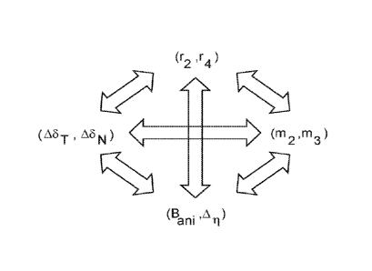
[0003] In the field of oil and gas exploration and recovery, analysis of
seismic
data obtained through seismic surveys provides valuable information about
structure
and physical parameters of subterranean rock formations. In a seismic survey,
a
source generates a seismic signal that propagates into the explored formation
and is, at
least partially, reflected at interfaces between a formation's layer having
different
acoustic impedances. The seismic signal is typically a compressional pressure
variation along the propagation direction (P-wave), but both P-waves and S-
waves (i.e.,
shear waves) may be detected. Seismic detectors record seismic data which
represent
Date Recue/Date Received 2021-09-27
CA 02943589 2016-09-22
WO 2015/145257
PCT/IB2015/000548
2
the detected waves. In fact, the recorded seismic data includes a convolution
of the
source wavelet (i.e., the signal's signature) and the formation's response
function.
Seismic data processing extracts the formation's response function, and then
various
parameters related to the explored formation. One way of expressing the
response
function is reflectivity, R, which for detected P-waves is Rpp. Reflectivity
may be
expressed as a function of the incidence angle, e, (which is defined in a
vertical plane
relative to the source position) and of the azimuth angle, 0 (which is defined
in a
horizontal plane around the source position). From the point of view of this
approach,
seismic data and reflectivity are the same.
[0004] Seismic data processing methods include azimuthal velocity
correction,
amplitude versus offset (AVO) analysis and inversion, amplitude versus offset
and
azimuth analysis (AVOAz) and inversion of conventional three-dimensional (3D)
seismic
data, and birefringence analysis of multicomponent 3D seismic data.
Reflectivity
characterizes subterranean properties and can serve as input to other
inversion
algorithms. For example, reflectivity can provide useful information regarding
the
anisotropy parameters of the subterranean formation, such as subsurface
fractures.
These anisotropy parameters may reveal shale plays, tight gas sands and coal
bed
methane, as well as carbonates in naturally fractured reservoirs. Note that
these
remarks are true also for seismic data in general. These characteristics and
parameters
.. are used to design and manage underground transportation systems,
foundations of
major structures, cavities for storage of liquids, gases or solids, etc. In
oil and gas
exploration, this kind of information is used for determining optimal
locations and
CG200156
3
orientations of wells (which may be vertical, inclined or deviated, and
horizontal), to
minimize wellbore instability and formation break-out. This information may
also be
used for stimulating the production of hydrocarbons by applying hydraulic
pressure on
the formation from the wellbore. The data inversions yield estimates of the
elastic
stiffnesses (velocities and anisotropic parameters) that can be used to
predict lithology,
porosity and the fluid content of the subsurface, as well as intensity and
orientation of
fractures in subterranean formations.
[0005] Conventional AVO inversions provide only band-limited fractional
elastic
parameters estimates with reduced resolution and quality (i.e., the bandwidth
of seismic
data is always less than the bandwidth of the desired reflectivities).
Conventional
AVOAz inversions are typically based on the near offset approximation of the
equation
set forth by ROger, A., 2002, "Reflection coefficients and azimuthal AVO
Analysis in
anisotropic media," SEG geophysical monograph series number 10: Soc. Expl.
Geophys (hereinafter "ROger"). ROger provides the equation showing the
amplitude R
with azimuth cp for narrow angles of incidence a However, this method has a
number of
limitations. For example, the near offset ROger equation is not theoretically
valid for the
case of two anisotropic half-spaces with different anisotropy orientation.
Further, there
is a 90-degree ambiguity associated with the estimate of the isotropy plane.
[0006] Recently, separating azimuthal AVO into AVO (Amplitude Versus
Offset) and
AVAz (Amplitude Versus Azimuth) has been achieved using Fourier coefficients
(FCs) as
described in U.S. Patent No. 8,792,303. This separation advantageously avoids
coupling
Date Recue/Date Received 2021-09-27
CA 02943589 2016-09-22
WO 2015/145257 PCT/IB2015/000548
4
between the isotropic and anisotropic properties.
[0007] Accordingly, it is desirable to enhance existing methods and
provide new
methods to extract anisotropic properties without the drawbacks and
limitations of
conventional methods.
SUMMARY
[0008] Methods and apparatuses according to some of the embodiments
use
statistical moments to separate AVO and AVAz and to extract anisotropy
parameters.
Under some assumptions, the moments are independent of the anisotropy
orientation.
The second and third central moments of azimuthal data are related to the
anisotropic
gradient and anellipticity variation, respectively. The moments can be
combined to
obtain more fundamental anisotropic properties, which can then be used to
obtain
unbiased estimates of the anisotropic gradient and orientation. Moments may be
further
used in combination with Fourier coefficients to help the interpretation and
yield
anisotropy model properties that closer relate data and model spaces.
[0009] According to an embodiment, there is a method for evaluating
anisotropy
parameters using statistical moments. The method includes obtaining seismic
data
considered as reflectivity values associated with pairs of incidence, 0, and
azimuth co
angles related to an explored formation, and calculating second central
moment, m2(0),
for at least two different incident angles and third central moment, m3(0),
for at least
zo one incident angle at a location within the explored formation using the
reflectivity
values. The method further includes obtaining tangential and normal weaknesses
for
the location using the calculated second and third central moments.
CA 02943589 2016-09-22
WO 2015/145257 PCT/IB2015/000548
[0010] According to another embodiment, there is an apparatus for
evaluating
anisotropy parameters from seismic data using statistical moments having an
interface
and a data processing unit. The interface is configured to obtain seismic data
considered as reflectivity values associated with pairs of incidence, e, and
azimuth co
5 angles related to an explored formation. The data processing unit
includes one or more
processors and is configured to calculate second central moment, m2(9), for at
least two
different incident angles and a third m3(9) central moment for at least one
incident angle
at a location within the explored formation using the reflectivity values. The
data
processing unit is further configured to determine tangential and normal
weaknesses for
the location using the calculated second and third central moments.
[0011] According to yet another embodiment, there is a computer
readable
recording medium non-transitorily storing executable codes which when executed
by a
computer make the computer perform a method for evaluating anisotropy
parameters
from seismic data using statistical moments. The method includes obtaining
seismic
data considered as reflectivity values associated with pairs of incidence, e,
and azimuth
9 angles related to an explored formation, and calculating second central
moment,
m2(e), for at least two different incident angles and third central moment,
m3(e), for at
least one incident angle at a location within the explored formation using the
reflectivity
values. The method further includes obtaining tangential and normal weaknesses
for
the location using the calculated second and third central moments.
BRIEF DESCRIPTION OF THE DRAWINGS
CG200156
6
[0012] The accompanying drawings illustrate one or more embodiments and,
together with the description, explain these embodiments. In the drawings:
[0013] Figure 1 is a polar graph of amplitude versus azimuth illustrating
seismic
data distributions;
[0014] Figure 2 includes an orthogonal graph of amplitude versus azimuth
illustrating the same seismic data distributions as in Figure 1, the graph
being framed by
histograms illustrating amplitude distributions (i.e., projections on y-axis
of the
orthogonal graph);
[0015] Figure 3 illustrates circles corresponding to the second central
moment
values in a 4th versus 2nd Fourier coefficient space;
[0016] Figure 4 illustrates hyperbolas corresponding to the third central
moment
values in the 4th versus 2nd Fourier coefficient space;
[0017] Figure 5 illustrates 2nd Fourier coefficient values in a second
versus third
central moment space;
[0018] Figure 6 illustrates 4th Fourier coefficient values in a second
versus third
central moment space;
[0019] Figure 7 schematically suggests relationships between coefficients
and
model spaces;
[0020] Figure 8 illustrates obtaining the tangential and normal weaknesses
using
second central moments for two angles of incidence and anellipticity variation
for one
angle of incidence in a tangential and normal weaknesses space;
Date Recue/Date Received 2021-09-27
CA 02943589 2016-09-22
WO 2015/145257
PCT/IB2015/000548
7
[0021] Figure 9 illustrates obtaining the tangential and normal
weaknesses using
third central moments;
[0022] Figure 10 is a flowchart of a method according to an
embodiment; and
[0023] Figure ills a schematic diagram of a seismic data processing
apparatus
according to an embodiment.
DETAILED DESCRIPTION
[0024] The following description of the exemplary embodiments refers
to the
accompanying drawings. The same reference numbers in different drawings
identify
the same or similar elements. The following detailed description does not
limit the
invention. Instead, the scope of the invention is defined by the appended
claims. The
following embodiments are discussed relative to analyzing seismic data to
estimate
elastic parameters of a subterranean formation.
[0025] Reference throughout the specification to "one embodiment" or
"an
embodiment" means that a particular feature, structure or characteristic
described in
connection with an embodiment is included in at least one embodiment of the
subject
matter disclosed. Thus, the appearance of the phrases "in one embodiment" or
"in an
embodiment" in various places throughout the specification is not necessarily
referring
to the same embodiment. Further, the particular features, structures or
characteristics
.. may be combined in any suitable manner in one or more embodiments.
[0026] Statistical moments of reflectivity provide another tool to
extract
anisotropic information from seismic data. Moments, which may be expressed as
non-
CA 02943589 2016-09-22
WO 2015/145257 PCT/IB2015/000548
8
linear combinations of FCs, provide the benefits of decoupling AVO and AVAz
reflectivity properties (e.g., avoiding leakage between isotropic and
anisotropic
properties estimation), and of decoupling the AVAz reflectivity properties
from the
anisotropy orientation. In one embodiment, the anisotropic gradient for small
incidence
angles is obtained from the second central moment using one angle of
incidence. In
another embodiment, the anellipticity variation is obtained using the fourth
FC and the
third central moment for only one angle of incidence. In yet another
embodiment, the
normal and tangential weaknesses variations (which yield the unbiased
anisotropic
gradient and unambiguous orientation) are obtained by combining the second (or
the
third) central moment defined at two angles of incidence and the anellipticity
variation
defined at one angle of incidence. Some templates are provided to illustrate
the
manner in which the moments and FCs data spaces relate to each other.
Anisotropic
templates are defined using a theoretical model to help with interpretation of
the data.
[0027] Moments are used in statistics to provide quantitative measures
of
.. distributions of points. There are different types of moments, including
raw moments,
central moments and normalized central (or standardized) moments. Raw moments
are
defined about the origin, and their discrete expression for an equi-
probability variable X
of dimension N is:
m,(ir) = Ekni= Xn (1)
N
where E denotes the expectation and n is the order of the moment.
[0028] The first raw moment mir) is the mean p, which is used in the
definition of
central moments:
CA 02943589 2016-09-22
WO 2015/145257 PCT/IB2015/000548
9
\n1 1
m,, = EkX ¨ j= ¨ ,u)" . (2)
N
[0029] The second central moment m2 is the variance, which is a
measure of the
dispersion or scatter of the data about the mean. The square root of m2 is the
standard
deviation a, which is used in defining standardized moments:
n
1 x-1N
mn E _______ - A, Z.s (3)
\ .1 lv-r 1=1 \
[0030] The third standardized moment m3' is called the skewness, which
is a
measure of the asymmetry or lopsidedness of a distribution. For a symmetrical
distribution, m3'= 0.
[0031] The mean, the variance, the skewness and higher order moments
can be
used to characterize any distribution. If AVAz amplitudes or reflectivities at
a given
angle of incidence are a set of points following a distribution (let us call
it "AVAz
distribution"), then statistical moments provide quantitative measures of the
shape of the
distribution. Figure 1 illustrates this concept with different types of
azimuthal anisotropy
for a given incidence angle. The points represent seismic amplitude
measurements for
a given incidence angle at different azimuths and the curves represent fit to
these points
with different level of accuracy. Line 110 is an isotropy fit, line 120 is
elliptical
anisotropy fit and line 130 is an anelliptical anisotropy fit. The radius of
each circle in
this polar graph corresponds to an amplitude value, and the azimuth angle 0
increases
counterclockwise from the rightmost point (trigonometric reference system).
[0032] Figure 2 includes a two-dimensional amplitude-versus-azimuth angle
graph (instead of Figure l's polar representation) of these fits, with line
210
CG200156
corresponding to 110, line 220 to 120 and line 230 to 130. If the curves are
projected
into histograms (i.e., projected on y-axis of the two-dimensional graph), the
isotropy fit is
a single bin 215, the elliptical anisotropy fit is a histogram 225, which is
symmetric
relative to the middle and peaking at the higher and lower values, and the
anelliptical
anisotropy fit is a histogram 235, which is an asymmetric distribution of
amplitude bins
with more lower values than higher values. The shape of such histograms
depends on
the azimuthal sampling of the amplitude and the size of the bins.
[0033] The mean is the same for the three fits. The variance is zero for
the
isotropy fit (110, 210) and non-zero for the elliptical (120, 220) and
anelliptical
anisotropy (130, 230). The skewness is zero for the isotropy fit (110, 210)
and elliptical
anisotropy fit (120, 220), but non-zero for the anelliptical isotropy fit
(130, 230). Thus,
moments carry information on azimuthal anisotropy. The variance is a measure
of the
dispersion or scatter about the mean. If the values are concentrated near the
mean
(which is the case for negligible azimuthal anisotropy), the variance is
small. In
contrast, if the values are distributed far from the mean (which is the case
for significant
anisotropy), the variance is large. The skewness seems to be sensitive to
anellipticity.
[0034] As stated in the article "Amplitude variation with azimuths (AVAz)
inversion based on linearized inversion of common azimuth sections" by IkeIle,
L.T.,
published in Seismic Anisotropy, pp. 601-644, SEG, Tulsa, the azimuthal PP
reflectivity,
Rpp, may be expressed using FCs for an incidence angle e and an azimuth angle
as:
Rõ( 0 , = ro(0)+r2(0)cos2(0 02) + r4(0)cos4(0 ¨ (4)
Date Recue/Date Received 2021-09-27
CA 02943589 2016-09-22
WO 2015/145257 PCT/IB2015/000548
11
where r, and 0; are respectively the magnitude and the phase of the ith FC.
[0035] Lines 210, 220 and 230 in Figure 2 may be reconstructed signal
using FC
of different orders. The constant amplitude fit (line 210) is using the 0th
order FC ro,
which is azimuthally invariant. The elliptical fit (line 220) is a 2nd order
FC approximation
using the terms ro and r2. The anelliptical fit (line 230) is a 4th order FC
approximation
using the terms ro, r2 and r4. As the order of the approximation increases,
the fit
improves as illustrated in Figure 1. For simplicity, the phase of the FCs is
assumed to
be the same (02= 04). As discussed In the article "Azimuth-dependent AVO in
reservoirs containing non-orthogonal fracture sets" by Sayers, C., and S.
Dean,
published in Geophysical Prospecting, 49, pp. 100-106, in 2001, this
assumption is valid
(1) in the case of an isotropic layer over an anisotropic layer where the
anisotropy of the
second layer is due to a single vertical fracture set, and (2) in the case of
two or more
non-orthogonal sets of vertical fractures when the normal to tangential
compliance ratio
is 1 and each fracture set has equal weight.
[0036] The first raw moment (or mean) of azimuthal data is simply the 0th
FC ro.
This term does not depend on the azimuth (i.e., it is an amplitude versus
offset, AVO,
term).
[0037] The second central moment m2 of azimuthal data may be expressed
as:
m2(1?õ(0,0))=m2(0)= 21(22(0)-Pr42()) = (5)
[0038] The third central moment m3 may be expressed as:
rn3(Rõ(0 ,0))= rn3(0)= ¨3r2 2 (9)r, (0). (6)
4
[0039] The second and third central moments are non-linear
combinations of the
CA 02943589 2016-09-22
WO 2015/145257 PCT/1B2015/000548
12
second and fourth FCs (i.e., r2and r4), which do not contain AVO reflectivity
properties.
Thus the AVO and AVAz problems are decoupled (similar to FCs). Since the
second
and third central moments do not depend on phase (i.e., the anisotropy
orientation), the
anisotropy orientation is decoupled from anisotropy intensity. As illustrated
in Figures 3
.. and 4, m2 is a circle of center (0,0) and radius (2m2(0))112 and m3 is a
hyperbola in the
FC data space (r2(9), r4(6)). These graphs' origins correspond to the isotropy
case. In
Figures 5 and 6, r2 and r4 are illustrated in (m2, m3) data space.
[0040] Under the assumption that anisotropy is due to a single set of
rotationally
invariant vertical fractures (i.e., HTI or azimuthal anisotropy), the Linear
Slip theory (as
.. set forth in the article, "Elastic behavior across linear slip interfaces,"
by Schoenberg
published in the Journal of the Acoustical Society of America, 68, pp. 1516-
1521, 1980),
defines a simple theoretical relationship between the seismic data and the
anisotropic
model properties, namely the normal and tangential weaknesses 5N and 5T. The
expressions of FCs in terms of Linear Slip properties are explained in the
article,
.. "Azimuthal Fourier Coefficients," by Downton, J., B. Roure, and L. Hunt,
published in the
Canadian Society of Exploration Geophysics Recorder, 36, #10, 22-36, in 2011.
Thus,
r2(9) and r4(e) are:
, 1
r2(9 )= + g(g- -OAS, tan 2 0 )sin2 0 (7)
2 ant
\
1-4( 9 )-1 Ari sin2 0 tan2 0 (8)
16
where
Barn = g(A6 ¨ xA6N) (9)
Ari = 2g(A8, ¨ N) (10)
CA 02943589 2016-09-22
WO 2015/145257 PCT/1B2015/000548
13
[0041] Ban; is the anisotropic gradient, q is the anellipticity (as
defined in the
article, "Estimation of fracture parameters from reflection seismic data ¨
Part 1: HTI
model due to a single fracture set," by Bakulin et al., published in
Geophysics, 65 (8),
pp. 1803-1817, 2000), and A represents the difference between the values above
and
below the interface. g is the square of the S-wave to P-wave velocity ratio of
the non-
fractured rock and x=1-2g. Figure 7 illustrates different parameter spaces
which can be
converted from one another. For example equations (9) and (10) indicate
conversion
from model space (MT A N) to model space (Bani, ,817). Equations corresponding
to
reverse transition (i.e., from model space (B01, Aq) to model space (A5T,
A5N)) are
easily obtained since equations (9) and (10) are linear. The weaknesses (My, A
N) are
sometimes considered more fundamental and less ambiguous properties than Bõ,,
Aq.
[0042] The 2nd and 4th FCs can be expressed in terms of weaknesses
variations
as:
'40 b(0)''A5,
(11)
1.-4(61)) c(0) d(0))A.5,
where
X \
(4 0 0) b 1 1 ¨ X 1 __ tan2 \
õ = ¨ g sin2 (9) 2x
I . (12)
c(61) AO)) 2 1 1
¨ tan2 (0) ¨ ¨4g tan2(0)
4
[0043] Mathematical manipulations of equations reveal that the second
central
momentum is an ellipse in (A5-, A5N) space. The matrix in equation (12)
transforms the
circle in the (r2,r4) space (equation 5) into an ellipse in (A5T, A5N) space
(equation 15).
CA 02943589 2016-09-22
WO 2015/145257 PCT/1B2015/000548
14
[0044] The following linear inversions allow obtaining anisotropic
properties (the
anisotropic gradient Ban, and the anellipticity variation Aq) from the second
and third
central moments, respectively. For small angles of incidence, the term
5in2(0)tan2(0)
becomes negligible in equations (7) and (8), and then by injecting equations
(7) and (8)
into equation (5), it follows that the anisotropic gradient Ban; is linearly
related to the
square root of the second central moment m2(e):
2r2 _________________________
Baõ, 2 õ (o). (13)
sin (e)
[0045] Due to the square root, this estimation of the anisotropic
gradient is
restricted to positive values only, similar to the near offset Ruger equation
or a simple
Fourier transform. Formula (13) can actually be extended to any even moments
(n=2,
4, 6, ...), i.e., the anisotropic gradient is linearly related to the nth root
of the nth moment
if n is even.
[0046] A simple Fourier transform gives the squared magnitude r;(6)
and r42(6)
but with no indication on the sign (see, e.g., equation (5) in the previously-
mentioned
article by Downton et al.). Based on equations (6) and (8), the third moment
has the
same sign as the anellipticity variation Aq and therefore r, (0). The
anellipticity variation
can hence be obtained from the third moment using a single angle of incidence
as:
64 1 1
Ari ¨ m(0). (14)
3 sin - 0 tan 2 0 r22 (0 )
[0047] Bõ; and 111-7 calculated using moments yields results similar
to the values
obtained using FCs (similarity which is a validation of the moments approach).
The
benefit of using moments is that the anellipticity is computed with only one
angle of
CA 02943589 2016-09-22
WO 2015/145257 PCT/1B2015/000548
incidence, while the calculation using FCs requires at least two angles of
incidence.
Using one angle of incidence instead of two is advantageous because
inconsistencies
between data corresponding to the two angles of incidence may be present due
to data
quality.
5 [0048] Estimating the tangential and normal weaknesses from the
moments is a
non-linear problem illustrated in Figure 8. Although a graphical method (with
ellipses
and lines) of obtaining (A5T, A5N) is explained below, the solution may be
obtained also
by solving equations, which may be computationally more efficient. In the
(.657-, A N)
space, the second central moment m2(e) defines an ellipse 810, all the points
on this
10 ellipse being possible solutions. In other words, having calculated the
second central
moment from azimuthal seismic data, it is impossible to determine which (MT,
MN)
couple is the real one along the ellipse. The third central momentum m3(0) can
then be
used to partially resolve this ambiguity. By providing an estimate of the
anellipticity
variation Ari, m3(6) linearly couples .657- and A5N through equation (10),
restricting actual
15 values (MT, .65N) to line 820. Thus, combining the second and third
central moments at
a single angle of incidence restricts the number of (MT, A5N) solutions to
two, i.e., the
points where line 820 intersects ellipse 810. Selecting one among the two
possible
solutions may be resolved by considering the second central moment defined at
another
angle of incidence as illustrated by ellipse 830. The intersection with
ellipse 830
indicates the real one among the two solutions. Since the existence and
uniqueness of
the solution are conditional upon the assumptions made, a confidence map
provided
alongside the results may be useful.
CA 02943589 2016-09-22
WO 2015/145257 PCT/1B2015/000548
16
[0049] Once L57- and MN are known, an unbiased expression of the
anisotropic
gradient Bard (not limited to positive values) is given by equation (9). The
estimation of
these anisotropic properties is done independently from the anisotropy
orientation.
Further, the phase of the 2' FC r2 may be used to obtain the symmetry axis
osym (i.e.,
the direction perpendicular to fractures). The Fourier transform yields the
magnitude of
the 2nd FC (limited to positive values) and its associated phase that wraps up
every 90
degrees (the phase of the nth FC is defined in [-Tr/(2n),+n-/(2n)]). The
actual phase can
be obtained by simply adding 90 degrees whenever the sign of the 2nd FC r2(6)
obtained
using equation (7) is negative. In other words, the 90-degree ambiguity on the
orientation is resolved by removing the ambiguity on the sign of the 2nd FC
magnitude.
[0050] The same technique as presented above using the second central
moments defined at two angles of incidence can also be used with the third
central
moments, providing the same results as described hereinafter relative to
Figure 9 and
formula 16. As illustrated in Figure 9, in the (L5T, MAI) space, the third
central moment
m3 for one angle defines a hyperbola 910, all the points on this hyperbola
being
possible solutions. The estimate of the anellipticity variation An linearly
couples A57-
and L5N through equation (10), restricting actual values (L5T, L N) to line
920. The
intersections of line 920 with hyperbola 910 yields two possible solutions 914
and 916,
which can be further selected using the third central moment m3 for another
angle.
[0051] Mathematically, if the 2nd and 4th FCs are expressed in terms of
weaknesses variations as set forth in equations 11 and 12,then the second
central
moment m2and third central moment m3 are:
CA 02943589 2016-09-22
WO 2015/145257
PCT/1B2015/000548
17
m, = 1 ¨2 06,2 (a 2 + C2 )+ (b2 + d2)+ 2AoTAS, (ab + cd)) (15)
3
[0052] m, = ¨4 kA8 ,3 a2 c + A5 õ21,2 d + AS ,2 A5 ,(2abc + a2 d)+ AS
, A5 ,2 (2abd + b2
(16)The above formalism can be extended to the sixth order FCs, with each FC
having
a different phase, according to the following formula:
1
=y ¨222 + r42 + r62)
3 , 3
m, = r2 r'cos 4(02 ¨04)+ ¨2 r2r4r6 COS(202 + 404 ¨ 66)
3
m4 = ¨kr4 + r4 + 1'1+ ¨1 r3 r6 cos 6(0, ¨06)+ (r2 r2 + r2 r7- + 1,211+
2 4 6 2 2 2 2 4 2 6 4 6
(17)
3 ...-2 r2,r4-1,6 COS (202 +66 ¨84)
75 4 3 2 2 5
ms = ¨ r2 r4 + 15 r2(-. r4 + 15 r2r4r6 cos 402 ¨04)+-8r4 r6- cos 12(04 ¨ )+
8 4
...15 1,41,6 + r2r:r6 + rz,r63)cos(2,02 +44 ¨66)
4 -
[0053] Figure 10 is a flowchart of a method 1000 for evaluating
anisotropy
parameters using statistical moments, according to an exemplary embodiment.
Method
1000 includes obtaining seismic data considered as reflectivity values, R(e,
(p),
associated with pairs of incidence, e, and azimuth go angles related to an
explored
lo formation, at 1010.
[0054] Method 1000 further includes calculating the second central
moment
m2(9), for at least two different incident angles and the third central
moment, m3(9), for
at least one angle of incidence, at a location within the explored formation
using the
reflectivity values, at 1020. The second and third central moments are
calculated using
formula (2), where X, are R(6, 9) values for different azimuth angles.
CA 02943589 2016-09-22
WO 2015/145257 PCT/1B2015/000548
18
[0055] Method 1000 then includes determining tangential and normal
weaknesses for the location using the calculated second and third central
moments for
the different incident angles, at 1030. In one embodiment, the tangential and
normal
weaknesses are determined by representing two of the calculated second moments
and
the anellipticity variation calculated from the third central moment in a two-
dimensional
space of the tangential and normal weaknesses. In another embodiment, the
tangential
and normal weaknesses are determined by representing two third moments and the
anellipticity variation, in a two-dimensional space of the tangential and
normal
weaknesses.
[0056] As previously described, a calculated second moment for an incidence
angle corresponds to an ellipse, and a calculated anellipticity variation for
the incidence
angle corresponds to a line in a two-dimensional space of the tangential and
normal
weaknesses. Parameters defining the ellipse and parameters defining the line
are
calculated using a square of the S-wave and P-wave velocity ratio, g, of the
non-
fractured rock and trigonometric functions of the incidence angle, e.
[0057] Method 1000 may also include calculating an anisotropic
gradient, Bani, for
small angles using the second central moment (e.g., using formula 13).
Alternatively or
additionally, method 1000 may include (A) inferring a 2nd Fourier coefficient
for an
incidence angle using a Fourier transform, and (B) evaluating an anellipticity
variation,
An, using the third central moment for the incidence angle, the inferred 2nd
Fourier
coefficient and the incidence angle (e.g., using formula 14).
CA 02943589 2016-09-22
WO 2015/145257 PCT/1B2015/000548
19
[0058] An apparatus 1100 capable of carrying out operations in
accordance with
the above-discussed methods is illustrated in Figure 11. Hardware, firmware,
software
or a combination thereof may be used to perform the various steps and
operations
described herein. Apparatus 1100 may include server 1101 having a central
processing
unit (CPU) 1102 which may be coupled to a random access memory (RAM) 1104 and
to
a read-only memory (ROM) 1106. Memory 1106 represents different types of
storage
media able to store executable codes. Thus, memory 1106 may be a programmable
ROM (PROM), an erasable PROM (EPROM), etc. Central processing unit 1102
includes one or more processors and may be configured to communicate with
various
internal and external components via input/output (I/O) circuitry 1108 and
bussing 1110
to provide control signals and the like.
[0059] Server 1101 may also include disk drives 1112, CD-ROM drives
1114,
and other hardware employed for reading and/or storing data, such as a DVD,
etc. In
one embodiment, software for carrying out the above-discussed steps may be
stored
and distributed on a CD-ROM 1116, removable media 1118 or other form of media
non-
transitorily storing information. The removable media may be inserted into,
and read by,
devices such as the CD-ROM drive 1114, disk drive 1112, etc. Server 1101 may
be
coupled to a display 1120, which may be any type of known display or
presentation
screen, such as LCD, plasma displays, cathode ray tubes (CRT), etc. Any of the
drives
may be a user interface configured to obtain (and provide to CPU 1102)
reflectivity
values associated with pairs of incidence, e, and azimuth go angles based on
seismic
data related to an explored formation.
CA 02943589 2016-09-22
WO 2015/145257 PCT/IB2015/000548
[0060] A user input interface 1122 including one or more user
interface
mechanisms such as a mouse, keyboard, microphone, touch pad, touch screen,
voice-
recognition system, etc., may be provided. Server 1101 may be part of a larger
network
configuration as in a global area network (GAN) such as the Internet 1128. CPU
1102
5 is configured (A) to calculate the second central moment, m2(0), for at
least two angles
of incidence and the third central moment, m3(0), for at least one incident
angle at a
location within the explored formation using the reflectivity values, and (B)
to determine
tangential and normal weaknesses for the location using the calculated second
and
third central moments.
10 [0061] Embodiments may be a computer program product which
implements
methods such as 1000. Accordingly, the embodiments may take the form of an
entirely
hardware embodiment or a combination of hardware and software. The computer
program product may be stored on a computer-readable storage medium having
computer-readable instructions embodied in the medium. Any suitable computer-
15 .. readable medium may be utilized, including hard disks, CD-ROMs, digital
versatile discs
(DVD), optical storage devices or magnetic storage devices such as floppy disk
or
magnetic tape. Other non-limiting examples of computer-readable media include
flash-
type memories or other known types of memories.
[0062] The disclosed exemplary embodiments provide methods and
apparatuses
20 for evaluating anisotropy parameters from seismic data using statistical
moments. It
should be understood that this description is not intended to limit the
invention. On the
contrary, the exemplary embodiments are intended to cover alternatives,
modifications
CA 02943589 2016-09-22
WO 2015/145257
PCT/1B2015/000548
21
and equivalents, which are included in the spirit and scope of the invention
as defined
by the appended claims. Further, in the detailed description of the exemplary
embodiments, numerous specific details are set forth in order to provide a
comprehensive understanding of the claimed invention. However, one skilled in
the art
.. would understand that various embodiments may be practiced without such
specific
details.
[0063] Although the features and elements of the present exemplary
embodiments are described in the embodiments in particular combinations, each
feature or element can be used alone without the other features and elements
of the
.. embodiments or in various combinations with or without other features and
elements
disclosed herein.
[0064] This written description uses examples of the subject matter
disclosed to
enable any person skilled in the art to practice the same, including making
and using
any devices or systems and performing any incorporated methods. The patentable
scope of the subject matter is defined by the claims, and may include other
examples
that occur to those skilled in the art. Such other examples are intended to be
within the
scope of the claims.