Note: Descriptions are shown in the official language in which they were submitted.
Time-Lapse Electromagnetic Monitoring
BACKGROUND
During oil and gas exploration and production, many types of information are
collected and analyzed. The information is used to determine the quantity and
quality of
hydrocarbons in a reservoir, and to develop or modify strategies for
hydrocarbon production.
One technique for collecting relevant information involves monitoring
electromagnetic (EM)
fields. Previous EM monitoring techniques do not appear to have adequately
addressed
techniques for time-lapse EM analysis, where EM survey data collected at two
different times
is analyzed to determine changes to a downhole environment. Efforts to improve
and to
efficiently obtain meaningful information from time-lapse EM analysis are
ongoing.
SUMMARY
In accordance with a first broad aspect, there is provided a time-lapse
electromagnetic
(EM) monitoring system for a formation, comprising at least one EM source, at
least one EM
field sensor to collect EM survey data corresponding to the formation in
response to an
emission from the at least one EM source, wherein the EM survey data includes
first EM data
collected at a first time and second EM data collected at a second time, and a
processing unit
in communication with the at least one EM field sensor, wherein the processing
unit
determines a perturbation tensor that defines a relationship between the first
EM data and the
second EM data, wherein the processing unit determines observed time-lapse EM
data based
on the first EM data and the second EM data, and wherein the processing unit
performs an
analysis of the observed time-lapse EM data to determine an attribute change
in an earth
model of the formation.
In accordance with a second broad aspect, there is provided a time-lapse
electromagnetic (EM) monitoring method for a formation, comprising emitting an
EM field,
collecting EM survey data corresponding to the formation in response to the
emitted EM field,
wherein the EM survey data includes first EM data collected at a first time
and second EM
data collected at a second time, determining observed time-lapse EM data based
on the first
EM data and the second EM data, wherein determining the observed time-lapse EM
data
comprises determining a perturbation tensor that defines a relationship
between the first EM
data and the second EM data, and analyzing the observed time-lapse EM data to
determine an
attribute change in an earth model of the formation.
CAN_DMS' \10866023112 1
CA 2944331 2017-09-25
BRIEF DESCRIPTION OF THE DRAWINGS
Accordingly, there are disclosed herein various time-lapse electromagnetic
(EM)
monitoring methods and systems, in which time-lapse EM data is directly
inverted to
determine an attribute change in an earth model. In the drawings:
FIGS. 1A-1C show illustrative time-lapse EM analysis scenarios.
FIG. 2 shows an illustrative logging-while-drilling (LWD) environment in which
EM
survey data may be collected.
FIG. 3 shows an illustrative wireline logging environment in which EM survey
data
may be collected.
FIG. 4 shows an illustrative monitoring well environment in which EM survey
data
may be collected.
FIGS. 5A and 5B show illustrative EM field sensor telemetry configurations.
FIG. 6 shows an illustrative time-lapse EM analysis method.
FIG. 7 shows a block diagram of an illustrative workflow with time-lapse EM
analysis operations.
It should be understood, however, that the specific embodiments given in the
drawings and detailed description below do not limit the disclosure. On the
contrary, they
provide the foundation for one of ordinary skill to discern the alternative
forms, equivalents,
and other modifications that are encompassed in the scope of the appended
claims.
DETAILED DESCRIPTION
The following disclosure is directed to time-lapse electromagnetic (EM)
monitoring
and analysis technology. The disclosed techniques employ at least one EM field
sensor to
collect EM survey data corresponding to a formation of interest, where the EM
survey data
includes first EM data collected at a first time and second EM data collected
at a second time.
A processing unit in communication with the at least one EM field sensor
determines
observed time-lapse EM data based on the first EM data and the second EM data.
The
processing unit performs an analysis of the observed time-lapse EM data to
determine an
attribute change in an earth model. In at least some embodiments, the
determined attribute
change corresponds to or is related to a change in resistivity. This attribute
change may be
used to update a resistivity model, a water saturation model, or other models
related to an
earth model. In some embodiments, the analysis of the observed time-lapse EM
data is a
direct inversion of time-lapse EM data, rather than separate inversions of EM
data collected
CAN_DMS 110866023112 2
CA 2944331 2017-09-25
at different times.
FIGS. 1A-1C show illustrative time-lapse EM analysis scenarios. FIG. IA shows
an
EM source 2A and an EM field sensor 4A at earth's surface 6 to conduct EM
surveys for
formation 8A. To conduct an EM survey, the EM source 2A emits an EM field, and
the EM
field sensor 4A detects an EM signal in response to the emitted EM field. At
time TI, the
detected EM signal is affected by properties of the formation 8A including
formation region
or volume 10A. The survey is repeated at time T1 + delay, when the detected EM
signal.is
affected by properties of the formation 8A including formation region or
volume 10B.
Assuming that the position of the EM source 2A and the EM field sensor 4A do
not change,
at least the movement of fluids in the formation 8A may cause the EM survey
data
corresponding to time TI and time TI -r delay to be different. The EM survey
data may also
change by varying the control parameters or position of the EM source 2A
and/or the EM
field sensor 4A. As long as relevant EM survey parameters (e.g., control
parameters, position,
etc.) are tracked, an estimate of changes in the EM survey data that are due
to movement of
fluids (or other formation attribute changes) can be obtained from time-lapse
EM analysis of
the EM survey data collected at time n and time n + delay. Such formation
attribute changes
are represented by A arrow 11A. As described herein, the delay value may vary,
though it is
expected to be in the range where measurable fluid front movement has occurred
(i.e., more
than l day and typically on the order of hundreds of days). A more detailed
explanation of
time-lapse EM analysis techniques is provided hereafter.
In the scenario of FIG. 1B, EM source 2B and EM field sensor 4B reside in a
borehole 12A to conduct EM surveys for formation 8B. For example, the EM
source 2B and
the EM field sensor 4B may be part of a LWD tool, a wireline logging tool, or
permanent
well installations (e.g., injection wells, production wells, or monitoring
wells). As the
arrangement of the EM source 2B and the EM field sensor 4B is different
compared to the
arrangement of EM source 2A and the EM field sensor 4A described in Fig. IA
(the EM
source 2B and EM field sensor 4B are downhole rather than at the surface), the
survey
measurements may be more sensitive to changes 11B in near-wellbore formation
regions 10C
and 10D. As with Fig. IA, EM survey data is collected by EM field sensor 4B in
response to
EM fields emitted by EM source 2B at time TI and time TI + delay. The
positioning of an
EM source and EM field sensors relative to each other and to a formation
determines which
formation region most strongly affects the collected EM survey data and the
related time-
lapse EM data. As desired, additional EM sources and/or EM field sensors
CAN_DMS: \ 108660231 \ 2 3
CA 2944331 2017-09-25
may be employed in scenarios of Figs. 1A-1B to expand the survey region.
Further, the
resolution of EM survey data can be adjusted by increasing or decreasing the
number of EM
sources and/or EM field sensors employed. Further, the spacing between EM
sources and/or
EM field sensors may vary.
In the scenario of FIG. IC, EM source 2C and EM field sensor 4C reside in
different
boreholes 12B and 12C to conduct EM surveys for formation 8C. For example, the
EM
source 2C and the EM field sensor 4C may each individually be part of a LWD
tool, a
wireline logging tool, or permanent well installations. Due to the arrangement
of the EM
source 2C and the EM field sensor 4C being different compared to the
arrangement of EM
sources and sensors in scenarios of Figs. 1A-1B (a cross-well arrangement is
shown rather
than a surface arrangement or single borehole arrangement), the survey
measurements may
be more sensitive to changes 11C in formation regions 10E and 10F. As with
Figs. 1A-1B,
EM survey data is collected by EM field sensor 4C in response to EM fields
emitted by EM
source 2C at time T1 and time T1 + delay.
The scenarios of Figs. 1A-1C are not intended to limit embodiments to a
particular
arrangement of EM sources and/or EM field sensors. For example, the scenarios
of Figs. 1A-
IC could be combined such that EM sources and/or EM field sensors are located
at the
earth's surface, at the seafloor, in a single borehole, and/or in multiple
boreholes. Further,
EM survey data may additionally or alternatively be collected using ambient EM
phenomena
in the downhole environment (a controlled EM source is not needed).
The EM sources and/or EM field sensor(s) used to collect EM survey data may be
temporarily or permanently positioned in a downhole environment. Temporary
positioning
CAN_DMS 110866023112 3a
CA 2944331 2017-09-25
CA 02944331 2016-09-28
WO 2015/160347 PCT/US2014/034416
EM sources and/or EM field sensors in a downhole environment may involve, for
example,
logging-while-drilling (LWD) operations or wireline logging operations with
one or more
EM sources and/or EM field sensors. Meanwhile, permanent positioning of EM
sources
and/or EM field sensors in a downhole environment may involve, for example,
permanent
well installations with one or more EM sources and/or EM field sensors.
While collecting EM survey data using the same EM source and EM field sensor
positions facilitates time-lapse EM analysis, it should be noted that EM
survey data collected
at different times may include EM data where the EM source position and/or the
EM field
sensor position has changed. In such case, collected position information for
the EM source
and/or the EM field sensors can be used to determine time-lapse EM data as
described herein.
The collection of EM survey data and the disclosed time-lapse EM analysis
techniques can be best appreciated in suitable application contexts such as an
LWD
environment, a wireline logging environment, and/or permanent well
installations.
FIG. 2 shows an illustrative drilling environment having a drilling platform
24 that
supports a derrick 14 having a traveling block 16 for raising and lowering a
drill string 32. A
drill string kelly 20 supports the rest of the drill string 32 as it is
lowered through a rotary table
22. The rotary table 22 rotates the drill string 32, thereby turning a drill
bit 40. As bit 40 rotates,
it creates a borehole 36 that passes through various formations 48. A pump 28
circulates
drilling fluid through a feed pipe 26 to kelly 20, downhole through the
interior of drill string 32,
through orifices in drill bit 40, back to the surface via the annulus 34
around drill string 32, and
into a retention pit 30. The drilling fluid transports cuttings from the
borehole 36 into the pit 30
and aids in maintaining the integrity of the borehole 36. Various materials
can be used for
drilling fluid, including oil-based fluids and water-based fluids.
As shown, logging tools 46 may be integrated into the bottom-hole assembly 42
near
the drill bit 40. As the drill bit 40 extends the borehole 36 through the
formations 48, logging
tools 46 may collect measurements relating to various formation properties as
well as the tool
orientation and various other drilling conditions. Each of the logging tools
46 may take the
form of a drill collar, i.e., a thick-walled tubular that provides weight and
rigidity to aid the
drilling process. For the present discussion, the logging tools 46 are
expected to include EM
field sensors and/or EM sources. The logging tools 46 may also include
position sensors to
collect position information related to EM survey data. In alternative
embodiments, EM
sources, EM field sensors, and/or position sensors may be distributed along
the drill string 32.
For example, EM sources, EM field sensors, and/or position sensor may be
attached to or
4
integrated with adapters 38 that join sections of the drill string 32
together. In such case,
electrical wires and/or optical fibers may extend through an interior of the
drill string 32,
through sections of the drill string 32, and/or in/through the adaptors 38 to
enable collection of
EM survey data and/or position data.
In some embodiments, measurements from the EM field sensors and/or position
sensors
are transferred to the surface using known telemetry technologies or
communication links.
Such telemetry technologies and communication links may be integrated with
logging tools 46
and/or other sections of drill string 32. As an example, mud pulse telemetry
is one common
technique for providing a communications link for transferring logging
measurements to a
surface receiver 49 and for receiving commands from the surface, but other
telemetry
techniques can also be used. In some embodiments, the bottom-hole assembly 42
includes a
telemetry sub 44 to transfer measurement data to the surface receiver 49 and
to receive
commands from the surface. In alternative embodiments, the telemetry sub 44
does not
communicate with the surface, but rather stores logging data for later
retrieval at the surface
when the logging assembly is recovered.
At various times during the drilling process, or after the drilling has been
completed, the
drill string 32 shown in FIG. 2 may be removed from the borehole 36. Once the
drill string 32
has been removed, as shown in FIG. 3, a wireline tool string 52 can be lowered
into the
borehole 36 by a cable 50. In some embodiments, the cable 50 includes
conductors and/or
optical fibers for transporting power to the wireline tool string 52 and
data/communications
from the wireline tool string 52 to the surface. It should be noted that
various types of
formation property sensors can be included with the wireline tool string 52.
In accordance with
the disclosed time-lapse EM analysis techniques, the illustrative wireline
tool string 52 includes
logging sonde 54 with EM sources, EM field sensors, and/or position sensors.
The logging
sonde 54 may be attached to other tools of the wireline tool string 52 by
adaptors 56.
In FIG. 3, a wireline logging facility 58 receives measurements from the EM
field
sensors, position sensors, and/or or other instruments of the wireline tool
string 52 collected as
the wireline tool string 52 passes through formations 48. In some embodiments,
the wireline
logging facility 58 includes computing facilities 59 for managing logging
operations, for
acquiring and storing measurements gathered by the logging sonde 54, for
inverting
measurements to determine formation properties, and/or for displaying
measurements or
formation properties to an operator. In some embodiments, the wireline tool
string 52 may be
lowered into an open section of the borehole 36 or a cased section of the
borehole 36. In a
CAN_DMS. \108660231\2 5
CA 2944331 2017-09-25
CA 02944331 2016-09-28
WO 2015/160347 PCT/US2014/034416
cased borehole environment, the casing may cause attenuation to signals that
are received by
the EM field sensors. However, the EM survey data can still be collected in a
cased borehole
environment, especially at low frequencies where attenuation due to casing is
low.
FIG. 4 shows an illustrative monitoring well environment. In FIG. 4, well 60
includes
borehole 61 containing a casing string 62 with a cable 78 secured to it by
bands 64. The
casing string 62 includes multiple tubular casing sections (usually about 30
foot long)
connected end-to-end by couplings. The cable 78 enables data and/or power
transmissions
and may correspond to an electrical conductor or optical fibers. Where the
cable 78 passes
over a casing joint 66, it may be protected from damage by a cable protector
67. The
remaining annular space in the borehole 61 may be filled with cement 76 to
secure the casing
string 62 in place and to prevent fluid flows in the annular space.
The well 60 is adapted to guide fluids 70 (e.g., oil or gas) from the bottom
of the
borehole 61 to earth's surface or vice versa. For example, fluids 70 can enter
the borehole 61
through uncemented portions or via perforations 72. Such perforations 72 near
the bottom of
the borehole 61 may extend through cement 76 and casing string 62 to
facilitate the flow of
fluid 70 from a surrounding formation (i.e., a "formation fluid") into the
borehole 61 and
thence to the surface via an opening at the bottom of or along production
tubing string 68.
Though only one perforated zone is shown for well 60, many wells may have
multiple such
zones, which enable production from different formations. Each such formation
may produce
oil, gas, water, or combinations thereof at different times. Alternatively,
the well 60 may
inject fluid into the borehole 61 and the different formations.
In FIG. 4, EM field sensors 74 couple to the cable 78 to enable collection of
EM
survey data that is conveyed to a surface interface 79 via the cable 78. In
some embodiments,
cable 78 may correspond to wired casing or wired production tubing with
couplers that provide
continuity of integrated electrical or optical paths. In such embodiments,
some or all of the
couplers may further include integrated EM field sensors 74. Alternatively,
cable 78 could be
arranged inside or outside of normal, metallic coiled tubing. Alternatively,
cable 78 could be
arranged on the inside of or attached to the outside of the production tubing
string 68. In at
least some embodiments, the EM field sensors 74 use wireless communications to
convey EM
field measurements to the surface or to a downhole interface that conveys the
measurement
received from the EM field sensors 74 to the surface. The EM field sensors 74
may in some
cases implement a mesh network to transfer data in a bucket-brigade fashion to
the surface.
The surface interface 79 may be coupled to a computer 80 that acts as a data
6
CA 02944331 2016-09-28
WO 2015/160347 PCT/US2014/034416
acquisition system and/or a data processing system that analyzes the EM field
measurements
to perform time-lapse EM analysis as described herein and/or other types of
data analysis. As
an example, the computer 80 (e.g., using processor 83) may process EM survey
data,
including first EM data collected at a first time and second EM data collected
at a second
time, to determine time-lapse EM data. The computer 80 also may perform an
inversion of
the time-lapse EM data to determine an attribute change in an earth model.
Further, the
computer 80 or another control system may direct control options for EM
sources (e.g., EM
sources 2A, 2B, 2C). Such control options may include waveform options,
current level
options, and timing synchronization between EM sources (e.g., EM sources 2A,
2B, 2C) and
EM field sensors (e.g., EM field sensors 4A, 4B, 4C).
As shown, the computer 80 includes a chassis 84 that houses various electrical
components such as processor 83, memories, drives, graphics cards, etc. The
computer 80
also includes a monitor 85 that enables a user to interact with the software
via a keyboard 86
or other input devices. Examples of input devices that may be used with or
instead of
keyboard 86 include a mouse, pointer devices, and touchscreens. Further, other
examples of
output devices that may be used with or instead of monitor 85 include a
printer. Software
executed by the computer 80 can reside in computer memory and on non-
transitory
information storage media 88. The computer may be implemented in different
forms
including, for example, an embedded computer installed as part of the surface
interface 79, a
portable computer that is plugged into the surface interface 79 as desired to
collect data, a
remote desktop computer coupled to the surface interface 79 via a wireless
link and/or a
wired computer network, a mobile phone/PDA, or indeed any electronic device
having a
programmable processor and an interface for I/0.
In different embodiments, the time-lapse EM analysis operations described
herein
may be performed by serial and/or parallel processing architectures. In some
embodiments,
the processing operations for time-lapse EM analysis may be performed remotely
from the
reservoir (e.g., cloud computers). For example, computers or communication
interfaces at the
reservoir site may be connected to remote processing computers via a network.
Accordingly,
computers at the reservoir site do not necessarily need high computational
performance.
Subject to network reliability, the time-lapse EM analysis operations
described herein may be
performed in real-time to update production, enhanced oil recovery (EOR)
operations, and/or
other operations.
FIGS. 5A and 5B show illustrative EM field sensor telemetry configurations
that
7
CA 02944331 2016-09-28
WO 2015/160347 PCT/US2014/034416
could be implemented in the environments of FIGS. 2-4. In FIG. 5A, sensor
groups 74A-74C
couple to cable 78 to perform EM field measurements and/or to convey EM field
measurements to a surface interface (e.g., interface 79). Each of the sensor
groups 74A-74C
may include orthogonal EM field sensors 90, 92, 94 (not shown for groups 74B
and 74C),
where sensor 90 is oriented along the z-axis, sensor 92 is oriented along the
x-axis, and
sensor 94 is oriented along the y-axis. In some embodiments, the cable 78
corresponds to one
or more electrical conductors to carry data and/or power. In such case, the EM
field sensors
90, 92, 94 may correspond to coils, electrodes, or another type of transducer
that generates or
modifies an electrical signal in response to an ambient EM field. The
generated or modified
electrical signal is transmitted to a surface interface (e.g., interface 79)
via cable 78, where its
characteristics can be interpreted to decode information about the EM field
sensed by one or
more of the sensors 90, 92, 94 in sensor groups 74A-74C.
In another embodiment, the cable 78 corresponds to one or more optical fibers
to
carry data and/or power. In such case, the EM field sensors 90, 92, 94
generate or modify a
light signal in response to sensing an ambient EM field. The generated or
modified light
signal is transmitted to a surface interface (e.g., interface 79) via one or
more optical fibers.
The surface interface converts the light signal to an electrical signal, whose
characteristics
encode information about the EM field sensed by sensor groups 74A-74C. It
should also be
understood that electro-optical converters may also be employed to change
electrical signals
to optical signals or vice versa. Thus, EM field sensors that generate or
modify a light signal
could be part of a system where cable 78 has electrical conductors. In such
case, the
generated or modified light signal is converted to an electrical signal for
transmission via
cable 78. Similarly, EM field sensors that generate or modify an electrical
signal could be
part of a system where cable 78 has optical fibers. In such case, the
generated or modified
electrical signal is converted to a light signal for transmission via cable
78.
In FIG. 5B, each of the sensor groups 74D-74F includes orthogonal EM field
sensors
90, 92, 94 (not shown for groups 74E and 74F), oriented as described for FIG.
5A. Further,
each of the sensor groups 74D-74F includes a wireless interface 96 to enable
communications
with a surface interface (e.g., interface 79). Each wireless interface 96 may
include a battery,
at least one wireless module, and a controller. In at least some embodiments,
the wireless
interfaces 96 are part of a wireless mesh in which short-range wireless
communications are
used to pass data from one wireless interface 96 to another until the data is
received by a
surface interface. As an example, a short-range wireless protocol that could
be employed by
8
CA 02944331 2016-09-28
WO 2015/160347 PCT/US2014/034416
each wireless interface 96 is Bluetooth . EM field sensor configurations such
as those shown
in FIGS. 5A and 5B may vary with respect to the position of sensor groups, the
types of
sensors used, the orientation of sensors, the number of cables/fibers used,
the wireless
protocols used, and/or other features.
FIG. 6 shows an illustrative time-lapse EM analysis method 160. The method 160
may be performed, for example, by one or more computers (e.g., computer 59 of
FIG. 3, or
computer 80 of FIG. 4) in communication with EM sources (e.g., EM sources 2A,
2B, 2C)
and/or EM field sensors (e.g., EM field sensors 4A, 4B, 4C). As
shown, the method
160 comprises collecting EM survey data including first EM data collected at a
first time and
second EM data collected at a second time (block 162). At block 164, observed
time-lapse
EM data is determined based on the first EM data and the second EM data. In at
least some
embodiments, the observed time-lapse EM data may be determined by defining a
relationship
between the first EM data and the second EM data. For example, the
relationship may be a
perturbation tensor or scalar value that defines a relationship between the
first EM data and
the second EM data. Further, the method 160 may include changing the
relationship as a
function of delay between the first and second times. For shorter delays
(e.g., less than a
couple of days), a scalar value may be used as the relationship metric. See
e.g., equation (17).
For medium delays (e.g., 2-7 days), a reduced perturbation tensor may be used
as the
relationship metric. See e.g., equation (16). For longer delays (e.g., more
than 7 days), a
perturbation tensor may be used as the relationship metric. See e.g., equation
(15).
At block 166, the observed time-lapse EM data is analyzed to determine an
attribute
change in an earth model. In at least some embodiments, the analysis step of
block 166 may
include comparing the observed time-lapse EM data with simulated time-lapse EM
data.
Further, the analysis step of block 166 may include relating the time-lapse EM
data to a
change in resistivity. Without limitation, the analysis step of block 166 may
subject attribute
changes of an earth model to one or more rock physics constraints and/or to
history-matched
constraints. Further, the analysis step of block 166 may apply a sensitivity-
based analysis to
determine the attribute change.
In at least some embodiments, the method 160 may include additional steps. For
example, the method 160 may additionally include determining position data
corresponding
to one or both of the first EM data and the second EM data, and using the
position data to
determine the observed time-lapse EM data. In this manner, differences in
position for EM
sources and/or EM field sensors may be accounted for.
9
CA 02944331 2016-09-28
WO 2015/160347 PCT/US2014/034416
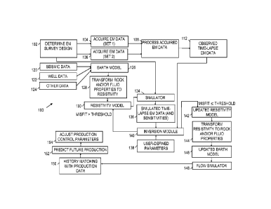
FIG. 7 shows an illustrative workflow 100 suitable for use with time-lapse EM
analysis operations. In workflow 100, the EM survey design is determined at
block 102. For
example, the EM survey design may include position, spacing, and control
parameters for
EM source and EM field sensors. At block 104, a first set of EM data is
collected. At a later
time, a second set of EM data is collected at block 106. The first and second
sets of EM data
are processed at block 108 to obtain time-lapse EM data 112. As will be
discussed in greater
detail below, the time-lapse EM data 112 may correspond to perturbed electric
field values.
The time-lapse EM data 112 is provided to inversion block 140.
The inversion block 140 also receives simulated time-lapse EM data 136 and
user-
defined parameters 138 as input. Examples of parameters 138 may include
adaptation step
sizes, constraints on model values, and criteria for terminating the inversion
process. The
simulated time-lapse EM data 136 is determined by a simulator 134 that
receives the EM
survey design 102 and a resistivity model 130 as input. In at least some
embodiments, the
simulator 134 also may provide sensitivity information to the inversion block
140. The
resistivity model 130 is initially derived from a transformation of an earth
model 126, which
in turn is obtained using seismic data 120, well data 122, and/or other data
124. The
transformation block 128 determines an initial resistivity model 130 based on
rock and/or
fluid properties of the earth model 126.
In at least some embodiments, the inversion block 140 compares the simulated
time-
lapse EM data 136 with the measured time-lapse EM data 112. If the misfit
(error) between
the simulated time-lapse EM data 136 and the time-lapse EM data 112 is greater
than a
threshold, the resistivity model 130 is updated, the EM measurement simulation
is repeated at
block 134, and the simulated time-lapse EM data is re-determined. An iterative
process of
comparing simulated time-lapse EM data 136 with the time-lapse EM data 112,
updating the
resistivity model 130, and re-simulating continues until the misfit between
the simulated
time-lapse EM data 136 and the time-lapse EM data 112 is less than or equal to
the threshold.
The result of this iterative process is an updated resistivity model 142 that
conforms to the
time-lapse EM data 112 to within a threshold tolerance.
At block 144, resistivity values of the updated resistivity model 142 are
transformed
to rock and/or fluid properties to obtain an updated earth model 146. The
updated earth
model 146 is used, for example, by a flow simulator 148 to predict future
production 152. In
at least some embodiments, the output of the flow simulator 148 is compared
with production
data by history matching block 150 to predict future production 152.
Production control
CA 02944331 2016-09-28
WO 2015/160347 PCT/US2014/034416
parameters are adjusted accordingly at block 154 to update production.
Thus workflow 100 represents an improved method of time-lapse EM analysis and
shows how it may be used to update production control parameters. A more
detailed
discussion incorporating specific time-lapse EM analysis modeling concepts is
now provided.
Generally, the electrical properties of a formation are heterogeneous and the
distribution of the electrical properties in an earth model of the formation
can be assumed to
be piecewise continuous. For example, a three-dimensional (3D) earth model
volume can be
constructed as the juxtaposition of volume elements populated by discrete
values of the
electrical properties and the EM fields and/or sensitivities modeled using a
3D numerical
simulator. For the purpose of 3D EM modeling, the 3D conductivity model can be
separated
into background (b) and anomalous (a) parts (having a spatial dependence
represented by the
coordinate vector r):
8(r) = 6-b (r) + ea (r), (1)
which can be complex, frequency-dependent, and be described by a second rank
tensor:
Fa a a
xx xy xz
a ¨ ayx ayy ayz , (2)
azx azy azz
which, due to energy considerations, is symmetric. It follows that Maxwell's
equations can
separate the electric and magnetic fields into background (b) and anomalous
(a) parts:
E(r) = Eb (r) + Ea(r), (3)
H(r) = Hb (r) + Hci(r), (4)
where the background fields are computed for the extraneous sources and the
background
conductivity model, and the anomalous fields are computed for scattering
currents in the
anomalous conductivity model. In EM modeling, the background conductivity
model may be
chosen such that the background fields can be evaluated analytically (e.g.,
homogenous
average conductivity) or semi-analytically (e.g., horizontal conductivity
layers) to avoid
subsequent numerical instabilities in the solution of the anomalous fields.
Further, Maxwell's equations may be solved in either of their differential or
integral
forms. For example, the EM fields can be written as the Fredholm integral
equations of the
second kind:
E(r') = Eb (r') + iv GE (r', r)o-c,(r)[Eb (r) + Ea (r)]d3r, (5)
H(r') = Hb (r') + iv dH(r', r)o-a(r)[Eb (r) + Ea (r)]d3r, (6)
11
CA 02944331 2016-09-28
WO 2015/160347 PCT/US2014/034416
where -dE,H is the electric or magnetic Green's tensor for the background
conductivity model.
In EM modeling, the background conductivity model may be chosen such that the
Green's
tensors can be evaluated analytically or semi-analytically to avoid subsequent
numerical
instabilities in the solution of the anomalous fields. See e.g., A Raiche, A
flow-through
Hankel transform technique for rapid, accurate Green's function computation:
Radio Science,
34 (2) 549-555 (2000). However, in some embodiments, the Green's tensors may
be
evaluated numerically for inhomogeneous background conductivity models.
While equations (5) and (6) are nonlinear, initially requiring the solution of
equation
(5) within the 3D earth model, equations (5) and (6) can be linearized by
assuming there
exists a linear relation between the anomalous and background electric fields
within the 3D
earth model:
Ea (r) = Fc(r)Eb(r), (7)
where k(e) is a second rank tensor:
fc = ky, kyy ky, , (8)
such that:
E(r') = Eb(e) + iv dE(r, r)o-c, (r) [1 + ic(r)]Eb(r)d3r, (9)
H(e) = Hb(rd) + iv dH(r', r)o-, (r) [1 + If (0]Eb (r)d3r.
(10)
The form of the tensor relating the anomalous and background electric fields
can be
quite arbitrary. Published literature shows that a prejudicial choice of the
form of the tensor k
can reduce equations (9) and (10) to a variety of approximations, such as the
Born
approximation, extended Born approximation, lo cal i zed nonlinear
approximation, quasi -
linear approximation, localized quasi-linear approximation, and quasi-linear
approximation.
See e.g., T. M. Habashy, R. W. Groom, and B. R. Spies, Beyond the Born and
Rytov
approximations: A nonlinear approach to electromagnetic scattering: Journal of
Geophysical
Research, 98 (B2), 1759-1775 (1993), and M. S. Zhdanov, Geophysical inverse
problems and
regularization theory: Elsevier, Amsterdam (2002). These various
approximations can
decrease computational complexity. However, these various approximations are
only valid
for relatively low conductivity contrasts.
Time-lapse EM modeling
12
CA 02944331 2016-09-28
WO 2015/160347 PCT/US2014/034416
For EM surveys with identical EM source and EM field sensor locations
conducted at
two different times (e.g., pre-production, during production, or combinations
thereof),
denoted by superscripts 1 and 2, equation (5) can be written as:
(e) = Eb (r') + .1.17 -dE(r', r)o-al(r)[Eb(r) + (0k/3r,
(11)
E2 (e) = Eb (r') + dE(r', r)o-g(r)[Eb(r) + Eci(r)1d3r,
(12)
Note that the background fields are constant between the two surveys, and the
time-lapse
change in conductivity manifests only in the change of the anomalous
conductivity from
o-al (r) to o-a2 (r).
The time-lapse EM response is hereby defined as the difference between
equations
(11) and (12):
Et 0.9 _ E2
= iv dE(r', r)fo-cli (r)[Eb (r) + (01 ¨ o-a2 (r) [Eb (r) + Ea2 (r)ild 3r
(13)
Time lapse EM data are measured as the difference between EM data from the two
EM
surveys conducted at different moments in time for the same EM source and EM
field sensor
locations. While it has been noted that survey repeatability is optimally
obtained from
permanent EM source and EM field sensor installations rather than from
repeated temporal
surveys as has been the focus of feasibility studies to date (see e.g., A.
Chuprin, D. Andreis,
and L. MacGregor, Quantifying factor affecting repeatability in CSEM surveying
for
reservoir appraisal and monitoring: SEG annual meeting, Expanded Abstracts
(2008)),
embodiments are not limited to permanent EM source and EM field sensor
installations as the
effects of differing transducer placements can often be determined and
accounted for.
The difficulty with equation (13) is that it is nonlinear with respect to both
the
anomalous conductivity and electric fields inside the 3D earth model at both
time periods.
Given this nonlinearity, it is the current belief that the time lapse EM
inverse problem must
be solved as two separate 3D EM inversion problems corresponding to the two
independent
EM surveys. See e.g., N. Black, G. A. Wilson, A. V. Gribenko, M. S. Zhdanov,
and E.
Morris, 3D inversion of time-lapse CSEM data based on dynamic reservoir
simulation of the
Harding field, North Sea: SEG Annual Meeting, Expanded Abstracts (2011), and
L. Srnka, J.
J. Carazzone, and D. A. Pavlov, Time lapse analysis with electromagnetic data:
U.S. Pat. No.
8,437,961. However, the present disclosure adopts a different approach.
13
CA 02944331 2016-09-28
WO 2015/160347 PCT/US2014/034416
While the following discussion is applied to electric f fields, it should be
appreciated
that a relationship between anomalous magnetic fields at different times also
exists and may
additionally or alternatively be used for time-lapse EM analysis.
In embodiments of this disclosure, it is assumed that there exists a relation
between
the anomalous electric fields at the two time periods:
Ea2(ro = RroEal(ro,
(14)
where ;10-9 is called a perturbation tensor, which is a second rank tensor
that can be proven
to always exist:
[
Axx Axy Axz
As = Ayx Ayy A yz =
Azx Azy Azz
(15)
Equation (14) is general, in that specific values, relations or functions need
not be
enforced upon the perturbation tensor, whose elements may be determined from a
deterministic function, from a linear minimization problem, or from a
nonlinear minimization
problem.
In some embodiments, the perturbation tensor can be reduced to be diagonally
dominant:
2-xx 0 0
A , [ 0 ilyy 01.
0 0 Az,
(16)
In some embodiments, the perturbation tensor can be reduced to be a scalar:
1 0 0
A = a[0 1 01 =at,
0 0 1
(17)
where I is the identity tensor.
The complexity of the perturbation tensor is related to the overall complexity
(i.e.,
non-linearity) of the time-lapse EM problem. For long time-lapse EM data under
certain
conditions (e.g., temporal monitoring from temporal installations), complete
solutions for
equation (15) may be required. For medium time-lapse EM data under certain
conditions
(e.g., temporal monitoring from permanent installations), equation (16) may be
sufficiently
accurate approximation for the perturbation tensor. For short time-lapse EM
data under
14
CA 02944331 2016-09-28
WO 2015/160347 PCT/US2014/034416
certain conditions (e.g., continuous monitoring from permanent installations),
equation (17)
may be a sufficiently accurate approximation for the perturbation tensor.
Without loss of generality, it follows that equation (14) reduces equation
(13) to the
integral equation:
[I ¨ RO]E,' (11 = fVE (r' Wo-cli(r) ¨ o-a2(r)}tEb(r) + [I ¨ A(r)[Ecil(r)P3r.
(18)
If:
P(r) = [I ¨ 21(r)[Eal(r), and
(19)
Ao-a(r) = (r) ¨
(20)
where P(r) is the electric field perturbation and Ao-a(r) is the change in
conductivity,
equation (18) can be re-written as:
P(r') = iv "dE(r', r)Ao-a(r)tEb(r) + P(r)}d3r,
(21)
which is recognized as a Fredholm integral equation of the second kind. It is
particularly
worth noting that the integral in equation (21) will only have contributions
from those
volumes of the 3D earth model where Ao-a(r) 0.
It is understood that in a reservoir with a waterflood, Ao-a(r) 0 where oil
and/or gas
has been displaced by water. It is also understood that in a reservoir with a
gas or CO2
injection, Ao-a(r) = 0 where oil has been displaced by if not mixed with gas
or CO2. It is
also understood that in an oil reservoir, Ao-a(r) 0 if the reservoir pressure
is not maintained
at or above bubble point as gas separates from oil. Such observations may
enable the
inversion process to particularly focus on the relatively small regions of the
model where
such changes might realistically occur. In any event, expressing the electric
field perturbation
in terms of the change in conductivity enables the use of some effective
linearization
approaches.
Example of linearization of the perturbation tensor: Time-lapse response
The following presents one example of a linearization of equation (18) to
solve for a
scalar perturbation tensor (17). Different methods of linearization can be
applied, and the
following example is not intended to limit the scope of the disclosure.
CA 02944331 2016-09-28
WO 2015/160347 PCT/US2014/034416
Assuming the perturbation tensor can be reduced to a scalar per equation (17)
and
with equation (20), equation (18) can be re-written as:
[1 ¨ A(e)]Eal(e) = fy GE(', r)Ao-a(r)(EB(r) + [1 ¨ A(r)]Ecil (r))d3r,
(22)
which can be expanded as:
[1 ¨ A(e)]E(e) = dE(r', r)10-a(r)Eb(r)d3r + f GE(r, r)Ao-a(r)[1 ¨
A(r)]Ect(r)d3r.
(23)
For EM modeling, the Green's tensor dE(r', r) exhibits a singularity when r' =
r
which must be avoided when computing the volume integrals in equation (23).
See e.g., T.
M. Habashy, R. W. Groom, and B. R. Spies, Beyond the Born and Rytov
approximations: A
nonlinear approach to electromagnetic scattering: Journal of Geophysical
Research, 98 (B2),
1759-1775 (1993). The result is that the dominant contributions to the
integrals on the right
hand side of equation (23) are from the observation points r that are proximal
to point r'. If
(r) is assumed to be a slowly varying function in the volume V such that A(e)
= (r),
then:
[1 ¨ A(r')]E(r') iv r)Ao-a(r)EB(r)d3r + [1 ¨
A.01] fif (r', r)Ao-c, (r)Eõ (r)d 3r. (24)
If:
EB (r') = fy "k(r, r)Acra(r)Eb (r)d3r,
(25)
EA (e) = 117 (r r)Ao-c, (Oki (r)d3r,
(26)
where EB (r') # 0 and EA (r') # 0 provided that o-a(r) # 0 for all r, equation
(24) can be
re-written as:
[1 ¨ A(r')]E(r') = EB (r') + [1 ¨ il(r0] EA (e),
(27)
and re-arranged to obtain:
[1 ¨ A(e)][Eõ1- (r) ¨ EA (r)] = EB (r').
(28)
With a scalar perturbation tensor, equation (28) can be reduced to a scalar
function by
calculating a dot product of both sides of equation (28). Assuming that EB
(r') # 0, the result
is:
16
CA 02944331 2016-09-28
WO 2015/160347 PCT/US2014/034416
1 ¨ 2t(e) = EB (r E'B (e)
[Egr')-EAVA-E*B(rT
(29)
where * denotes the complex conjugate. Re-arranging equation (29) results in
an expression
for the scalar perturbation tensor:
2t(e) = 1
E (r ICE (V) [E(r')-EAV)-EB(r)].E*BV)
[E(r')-EA(r')].E*B(r') [Eld(C)-EAVA=q(C)
(29)
assuming that [Ea' (r') ¨ EA (r')] = E( r') # 0, and where Eal EB (0, and
EA (r') all have
known (or calculated) values. The advantage of equation (29) is that the
scalar perturbation
tensor can be evaluated quasi-analytically.
Example of linearization of the perturbation tensor: Time-lapse sensitivities
For inversion, the Frechet derivatives (or sensitivities) of equation (18) may
be
calculated with respect to the time lapse change in conductivity, Ao-a(r). The
following
presents one example of a linearization of equation (18) to solve for a scalar
perturbation
tensor (17). With equation (20), equation (18) can be re-written as:
013(0 a
15[6.0-a ()] = a [A ca (01v GE(r',06,0-a(r)tEb(r) + [1¨ 2t(r)]Ela(r)id3r,
(30)
With:
daE(V,r) OEb(r) OE(r)
= 0,
a [Auct(r)] a [Aga (0] a [Aga (0]
(31)
equation (30) reduces to:
aP(r0
a [Aga (01
iv CE(r', Eb (r) + [1 ¨ A(r)]Eia(r)}d3r ¨f,, dE(r', r)Ao-a(r) "(I) a[)1
Va(r)d3r. (32)
Further, Quasi-Born sensitivities can be written as:
F(12B(e) = dE(r', r)fEb(r) + E1a(r)}d3r,
(33)
and equation (32) simplifies to:
aP(r0
=FQBi (r') -dE(rr, r) {2t(r) + Ao-a a16 )]
(r) ____________________________________________ Eal- (r)d3r.
a[Aaa(0] ,ga(r
(34)
17
CA 02944331 2016-09-28
WO 2015/160347 PCT/US2014/034416
The advantage of an equation such as equation (34) is that the Frechet
derivatives (or
sensitivities) can be evaluated with minimal computational expense since all
variables in
equation (34) are known from modeling (18), or can be easily evaluated from
known
variables (e.g., __ (32..(r) can be simply evaluated from the chain rule
differentiation of
a [Ace/ (r)]
equation (29)).
Rock physics constraints on formation conductivity
The effective conductivity of a reservoir formation can be frequency-dependent
(i.e.,
inclusive of dielectric and/or induced polarization effects) and either scalar
or anisotropic.
The effective conductivity can be expressed through an -effective medium"
model and
described in terms of rock and fluid properties such as porosity,
permeability, fluid
(oil/gas/water) saturation, and rock matrix composition. These effective
medium models can
be derived analytically, semi-analytically, or empirically. In waterflood
monitoring, the water
saturation is the most critical fluid parameter. Since the time-lapse change
in conductivity can
be related to the time-lapse change in water saturation via a continuous and
differentiable
function:
Ao-a(r) = f [AS, (r)],
(35)
it follows that the sensitivities with respect to the time-lapse change in
water saturation can
be calculated as:
a a[6.act (r)] a
[ASw (r)] a [6,Sw(r)] a [Ao- a (r)]
(36)
It is understood that the effective conductivity can also be inclusive of
macro-scale rock and
fluid properties, such as natural and/or induced fractures and/or proppants
and/or other
introduced fluids. For example, the effective (scalar) conductivities of
reservoir formations
have long been described by the empirically-derived Archie's Law:
ae = af (km57'
(37)
which relates the effective (scalar) conductivity cie of a porous medium as a
function of the
tortuosity factor a, fluid conducitivity o-f, porosity 0 , cementation
exponent m, fluid
saturation Sf, and saturation exponent n; assuming that the rock matrix is non-
conductive.
18
CA 02944331 2016-09-28
WO 2015/160347 PCT/US2014/034416
Archie's law is widely accepted as being relevant for sandstone reservoirs
absent of clay
minerals.
Assuming a clean sandstone reservoir formation (n = 1), and that the
conductivity of
brine is (typically) much larger than the conductivity of oil, this implies
that the time-lapse
change in conductivity can be expressed as:
= ¨a Ciw (r) AS, (r) ¨ ¨a a, m (OAS (r) ¨a m (r) AS, (r),
(38)
where all change in the effective conductivity can be attributed to brine
displacement of oil
along the oil-water contact. The conductivity of brine can be estimated from
injection water
analysis, and the porosity known a priori from reservoir models. From equation
(38), a
derivative is obtained:
a [Aga (r)]1
= O m (a
0 [6,Sw (01 a
(39)
such that
a
= (r) a
dp,Sw(r)] a [6,0a (0] =
(40)
For example, equation (32) can be re-written as:
aP(r')= ) 1 aP(e)
cj
0 [6,Sw (01 a
(41)
which enables onc to invert time-lapse EM data for the change in water
saturation.
History-matched constraints
For the purpose of waterflood monitoring, the inversion may be subjected to
the
ancillary constraints that the total change in mass of water in the updated
water saturation
model is conserved:
mõ =
(42)
where mõ is the total mass of water injected (known from production data), p,
is the water
density (which may vary with salinity and temperature), and that the water
saturation in the
model can only increase:
S( r) > 0,
(43)
19
CA 02944331 2016-09-28
WO 2015/160347 PCT/US2014/034416
and where the water saturation is bound:
0 S(r) 1 ¨ (r),
(44)
where S is the residual oil saturation.
Other considerations
In different embodiments, the method can be applied to the simultaneous
modeling,
inversion, and/or imaging of time-lapse EM data acquired during at least two
different times.
In some embodiments, workflows encapsulating the disclosed time-lapse EM
analysis
techniques can be inclusive of prior art modeling, inversion, and/or imaging
methods of EM
survey data collected at two or more different times. Such workflows can
ensure data quality
control, system calibration, and may eliminate cumulative errors since any
systematic error in
the time-lapse EM measurements will result in increasing absolute errors in
the time-lapse
EM data.
In different embodiments, the temporal and/or permanent emplacement of EM
sources and/or EM field sensors is arbitrary, and such components may be
placed on the
surface, on the seafloor, or in at least one borehole. Further, the type of EM
source used in
the EM survey is arbitrary, and may include any electric and/or magnetic
source types.
Further, the type of EM field sensor used in the EM survey is arbitrary, and
may include any
electric and/or magnetic field sensor types such as but not limited to coils,
electrodes, and
fiber optic sensors.
The earth models mentioned herein can be constructed using industry-standard
earth
modeling software (e.g., DecisionSpace0) and workflows from available well,
seismic, and
production data. Further, rock and fluid attributes of the earth models can
include porosity,
permeability, oil saturation, gas saturation, and water saturation. The EM
attributes of the
earth models can include resistivity, conductivity, permittivity,
permeability, chargeability,
and other induced polarization (IP) parameters. Further, the EM attributes of
the earth models
can be either isotropic or anisotropic.
In some embodiments, the EM attributes of the earth model are populated from
the
interpolation and/or extrapolation of well-based resistivity data within well-
tied seismic-
based structural models. In these embodiments, the interpolation and/or
extrapolation
algorithms may be based on geostatistical methods. Also, the well-based
resistivity data can
be derived from any one or a combination of LWD resistivity or dielectric
data, wireline
resistivity or dielectric data, open-hole resistivity or dielectric data,
cased-hole resistivity or
CA 02944331 2016-09-28
WO 2015/160347 PCT/US2014/034416
di el ectric data, through-casing resistivity or di electric data, single-
component resistivity or
dielectric data, and multi-component resistivity or dielectric data.
In some embodiments, the EM attributes of the earth models can be related to
the rock
and fluid attribute of the earth models. Further, different attributes of the
earth model may be
assigned to different grids and/or meshes as required for different
simulators. For example,
the EM simulator will generally operate upon a different grid and/or mesh to a
multi-phase
flow simulator. In these embodiments, the attributes of one grid and/or mesh
can be upscaled,
down-scaled, interpolated and/or extrapolated to populate the attributes of
another grid and/or
mesh. Attribute transforms (e.g., calculating resistivity from porosity and
water saturation)
can be applied before or after such interpolations and/or extrapolations.
The workflows described herein can be implemented as either stand-alone
software or
integrated as part of a commercial earth modeling software (e.g.,
DecisionSpace) through an
application programmable interface (API). Further, the dimensionality of the
earth model and
related EM simulator (e.g., 1D, 2D, 3D) is based on the interpreter's
prejudice and/or
requirement for solving particular reservoir monitoring problems. In some
embodiments, an
earth model of a lower dimensionality (e.g., 1D or 2D) can be extracted from
an earth model
of a higher dimensionality (e.g., 3D).
The EM simulator can be based on any combination of analytical, semi-
analytical,
finite-difference, finite-volume, finite-element, boundary-element, and/or
integral equation
methods. The simulation methods may be implemented in Cartesian, cylindrical
and/or polar
coordinates. Further, the EM simulator can be programmed on serial and/or
parallel
processing architectures. Likewise, EM modeling, inversion, and/or imaging
algorithms may
be implemented using software programmed for serial and/or parallel processing
architectures. The processing of the EM modeling, inversion, imaging, and/or
related
functions may be performed remotely from the reservoir, where computers at the
reservoir
site are connected to the remote processing computers via a network (e.g.,
cloud computers).
In such case, computers at the reservoir site should have high network
reliability, but do not
need high-computational performance, since EM modeling, inversion, and/or
imaging can be
performed by remote computers in real-time or near real-time.
In at least some embodiments, the disclosed time-lapse EM analysis can be used
to
perform joint inversion of time-lapse EM data with any other geophysical
(e.g., seismic,
time-lapse seismic, gravity, time-lapse gravity) and/or production (e.g.,
multi-phase flow)
data. Further, the disclosed time-lapse EM analysis can be used for reservoir
management
21
CA 02944331 2016-09-28
WO 2015/160347 PCT/US2014/034416
systems, inclusive of intelligent completions and/or intelligent wells, for
improved
production enhancement.
In at least some embodiments, the disclosed time-lapse EM analysis can be used
with
a permanently installed fiber optic-based EM reservoir monitoring system.
Further, the
disclosed time-lapse EM analysis can be used with a permanently installed EM
cement
monitoring system for characterizing cement cure state and integrity. Further,
the disclosed
time-lapse EM analysis has relevance to drilling and wireline formation
evaluation
applications, and/or other EM-based monitoring applications.
The disclosed time-lapse EM analysis enables directly modeling, inverting
and/or
imaging upon time-lapse EM data to recover the time lapse changes in
conductivity
(resistivity), water saturation, hydrocarbon saturation, and carbon dioxide
saturation
attributes of earth models. Such time-lapse EM analysis is compatible with
static, quasi-
static, and dynamic earth models. Updates to such earth models may be
performed in real-
time.
In at least some embodiments, the disclosed time-lapse EM analysis can be
applied to
any surface, borehole, borehole-to-surface, cross-borehole, or marine EM
method used for
temporal and/or permanent reservoir monitoring. The disclosed time-lapse EM
analysis can
be used to monitoring different types of fluid such as oil, gas, water, carbon
dioxide, water-
based mud, oil-based mud, spacer, and/or cement. Further, the disclosed time-
lapse EM
analysis may be used with oil and gas production, carbon sequestration,
enhanced oil
recovery (EOR) operations (waterflooding and/or CO2 injection), and/or
groundwater
operations.
For the disclosed time-lapse EM analysis, EM survey data may be acquired from
at
least two temporal surveys, where the position of EM source and/or EM field
sensors has
changed (e.g., cross-borehole EM, marine EM). In such case, interpolation,
extrapolation,
and/or integral transforms can be applied to redatum measured EM data from at
least one
temporal survey to the same EM source and/or EM field sensor positions of at
least one other
temporal survey such that time-lapse EM data between the at least two temporal
EM surveys
can be computed.
Embodiments disclosed herein include:
A: A tim e-1 ap se electromagnetic (EM) monitoring systems for a formation
that
comprises at least one EM source, and at least one EM field sensor to collect
EM survey data
corresponding to the formation in response to an emission from the at least
one EM source, and a
22
CA 02944331 2016-09-28
WO 2015/160347 PCT/US2014/034416
processing unit in communication with the at least one EM field sensor. The EM
survey data
includes first EM data collected at a first time and second EM data collected
at a second time.
The processing unit determines observed time-lapse EM data based on the first
EM data and
the second EM data. The processing unit performs an analysis of the observed
time-lapse EM
-- data to determine an attribute change in an earth model.
B: A time-lapse electromagnetic (EM) monitoring method for a formation that
comprises emitting an EM field and collecting EM survey data corresponding to
the
formation in response to the emitted EM field. The EM survey data includes
first EM data
collected at a first time and second EM data collected at a second time. The
method also
-- comprising determining observed time-lapse EM data based on the first EM
data and the
second EM data, and analyzing the observed time-lapse EM data to determine an
attribute
change in an earth model.
Each of the embodiments, A and B may have one or more of the following
additional
elements in any combination: Element 1: the processing unit determines the
observed time-
-- lapse EM data using a perturbation tensor that defines a relationship
between the first EM
data and the second EM data. Element 2: the relationship is scalar. Element 3:
the analysis
corresponds to an inversion based on a comparison of the observed time-lapse
EM data with
simulated time-lapse EM data, wherein the inversion minimizes an error between
the observed
time-lapse EM data and the predicted time-lapse EM data subject to constraints
imposed on an earth
-- model. Element 4: further comprising at least one position sensor to
determine position data
corresponding to one or both of the first EM data and the second EM data,
wherein the
processor uses the position data to determine the observed time-lapse EM data.
Element 5:
the analysis relates the observed time-lapse EM data to a change in
resistivity. Element 6: the
determined attribute change is used to update a resistivity model or water
saturation model.
-- Element 7: the inversion subjects the attribute change to one or more rock
physics
constraints. Element 8: the inversion subjects the attribute change to history-
matched
constraints. Element 9: the inversion applies a sensitivity-based analysis to
determine the
attribute change. Element 10: further comprising a logging-while drilling
(LWD) string or a
wireline tool string to temporarily position the at least one EM source or the
at least one EM field
-- sensor in the formation. Element 11: further comprising a permanent well
installation to
permanently position the at least one EM source or the at least one EM field
sensor in the
formation.
23
CA 02944331 2016-09-28
WO 2015/160347 PCT/US2014/034416
Element 12: determining the observed time-lapse EM data comprises assigning a
relationship between the first EM data and the second EM data. Element 13:
further
comprising changing the defined relationship as a function of delay between
said first and
second times. Element 14: said analyzing comprises comparing the observed time-
lapse EM
data with simulated time-lapse EM data and minimizing an error between the
observed time-lapse
EM data and the predicted time-lapse EM data subject to constraints imposed on
an earth model.
Element 15: further comprising determining position data corresponding to one
or both of the
first EM data and the second EM data, and using the position data to determine
the observed
time-lapse EM data. Element 16: said analyzing comprises relating the observed
time-lapse
EM data to a change in resistivity and subjecting the attribute change to one
or more rock
physics constraints. Element 17: said inverting comprises relating the
observed time-lapse
EM data to a change in resistivity and subjecting the attribute change to
history-matched
constraints. Element 18: said analyzing comprises relating the observed time-
lapse EM data
to a change in resistivity and applying a sensitivity-based analysis to
determine the attribute
change.
Numerous other variations and m o di fi cations will become apparent to those
skilled in
the art once the above disclosure is fully appreciated. It is intended that
the following claims
be interpreted to embrace all such variations and modifications where
applicable.
24