Note: Descriptions are shown in the official language in which they were submitted.
SYSTEM AND METHOD FOR SPATIALLY IMAGING AND CHARACTERIZING
PROPERTIES OF ROCK FORMATIONS USING SPECULAR AND NON-SPECULAR
BEAMFORMING
E THE INVENTION
[0001] This disclosure isr FIELD
OF
related to he field of seismic imaging of subsurface rock
formations. More specifically, the disclosure concerns locating spatial
position of
seismic diffractors in the subsurface from a wellbore, either while the
wellbore is being
drilled or thereafter.
BACKGROUND
[0002] Wellbore drilling through subsurface rock formations may be
performed for the
purpose of positioning such wellbores or parts thereof in formations
containing useful
materials such as hydrocarbons or other minerals. Structures of the subsurface
formations, and to some extent the composition of the formations may be
determined by
reflection seismic surveying techniques known in the art.
[0003] As a practical matter, reflection seismic surveying known in the art
for
determining structural and/or compositional features in the subsurface tend to
emphasize features identifiable from specular reflections. It is known in the
art that
certain features in subsurface formations act as diffractors or scatters of
seismic energy.
In some cases, geologic properties associated with such diffractors may
present drilling
hazards or the properties of such diffractors may be economically useful. It
is desirable
to be able to determine the spatial position of such diffractors.
[0004] U.S. Patent No. 9,476,997 issued to Pace and Guigne discloses a
method locating
diffractors in the subsurface. Such disclosed method for locating diffractors
in
subsurface formations includes actuating at least two seismic energy sources
at spaced
apart locations. Seismic energy is detected in the formations resulting from
actuation of
the two sources. Signals corresponding to the detected seismic energy are
processed to
remove components related to direct arrivals from each source. Arrival times
of seismic
energy in the signals corresponding to energy diffracted from at least one
diffractor are
CA 3035192 2019-02-28
identified. The at least one is located diffractor in a plane using the
identified arrival
times.
[0005] There continues to be a need for improved methods for imaging
diffractors in
subsurface formations using seismic and/or acoustic signals.
SUM MARY
100061 A method for imaging non-specular seismic events in a volume of
Earth's
subsurface includes entering as input to a computer signals detected by a
plurality of
seismic sensors disposed at least one of above or within the volume in
response to
actuation of at least one seismic energy source at least one of above or
within the volume;
in the computer, determining presence of a specular event in the detected
signals and if a
specular event is determined, a) in the computer, using the determined
specular event to
calculate a normal vector at selected points in the volume; b) in the
computer, using the
normal vectors, the detected signals and a model of seismic velocity as input
to
beamforming to obtain specular and non-specular representations of the volume;
if a
specular event is not determined, beamforming the detected seismic signals to
generate
an image of a non-specular event in the volume, the beamforming comprising
associating
specific amplitudes in the detected seismic signals with specific locations
within the
volume; in the computer, carrying out correlations of measured seismic
properties
measured in a wellbore with at least one of the specular or non-specular
events; and in
the computer, displaying the correlations.
100071 Some embodiments further comprise calibrating the seismic
attributes to formation
properties using measurements from samples of rock formations obtained from a
wellbore
and using the calibrated seismic attributes to determine the formation
properties at
positions in the volume spaced apart from the wellbore.
100081 Some embodiments further comprise determining at least one of
structure of,
mineral composition of and fluid content of a formation using seismic
attributes
determined from the non-specular reflections data sets.
[0009] In some embodiments, the beamforming comprises implementing, /(x0,
x1, x2) =
(s,r) E (s, r, t) o (Ei Er(s,r,x0,x1,x2) w( s, r, xo,x1,x2) (t
(i) (s, r, xo, xi., x2)))
2
Date Recue/Date Received 2021-07-29
wherein:
F(s,r,x 0,x 1,x 2) represents the space all ray-paths connecting source
location s
to image point I (x 0,x 1,x2) to sensor locations r;
I(x 0,x 1,x 2 ) represents the output (e.g., scattering intensity,
reflectivity,
attenuation) at (x 0,x 1,x2 ) location, where the output depends on input data
type and is
not a proxy for a property under assessment;
represents the collection of all source-sensor pairs;
kP(s,r,t) represents a trace, that is, signals detected by a sensor at
location r, due to
source at location s, with t representing that senor's event detection time. A
trace may be
extended to infinity by padding with zeros before and after the detection
time;
6 represents Dirac distribution (continuous-time signal representation) or
Kronecker delta (discrete-time signal representation);
0 represents 1-dimensional convolution evaluated at 0 (zero);
(I) i (s,r,x 0,x 1,x2 ) represents the function which returns travel time from
source
location s to image point I (x 0,x 1,x2) to sensor location r along a specific
ray-path,
Kw i (s,r,x)1 0,x 1,x 2) represents a weight function which embodies,
amplitude
transmission loss due signal travel from source to image point to receiver,
normalization
correction due to variable summation count, and specularity or non-specularity
condition
(pass-reject) based on desired output.
100101 In some embodiments, the determining a specular event comprises
reflection
seismic image processing.
[0011] In some embodiments, the reflection seismic image processing
comprises prestack
time migration or prestack depth migration.
100121 In some embodiments, inputs to the beamforming comprise the
detected signals,
spatial distribution of velocity in the volume and a normal vector at each of
a plurality of
points in the volume
3
Date Recue/Date Received 2021-07-29
100131 In some embodiments, the spatial distribution of velocity is
determined by
reflection seismic imaging velocity analysis.
[0014] In some embodiments, the reflection seismic image processing
comprises prestack
time migration or prestack depth migration.
100151 In some embodiments, the normal vector is determined by best fit
curve matching
a plurality of points in the volume.
[0016] Some embodiments further comprise adjusting the trajectory of a
well based on the
image of the non-specular event.
100171 Some embodiments further comprise using the input to beamforming to
transmit a
beamformed seismic signal.
[0018] Another method for imaging non-specular seismic events in a volume
of Earth's
subsurface includes: sensing seismic signals using a plurality of seismic
sensors disposed
at least one of above or within the volume in response to actuation of at
least one seismic
energy source at least one of above or within the volume; determining presence
of a
specular event in the detected signals and if a specular event is determined:
determining
from the seismic signals inputs for beamforming; and transmitting a beamformed
seismic
signal based on the determined inputs; and absent detecting a specular event,
displaying an
image of a non-specular event in the volume, the image of the non-specular
event generated
by beamforming the detected seismic signals, the beamforming the detected
seismic signals
comprising associating specific amplitudes in the detected seismic signals
with specific
locations within the volume.
BRIEF DESCRIPTION OF THE DRAWINGS
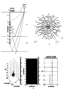
[0019] FIG. lA shows a seismic energy source and receiver array that may
be used in some
embodiments.
4
Date Recue/Date Received 2021-07-29
100201 FIG. 1B shows another possible implementation having even greater
source
focusing capability than the example shown in FIG. 1A.
[0021] FIG. 1C shows a beam pattern for a possible implementation of a
source and sensor
array.
100221 FIG. 2 shows a flow chart of an example method according to the
present
disclosure.
4a
Date Recue/Date Received 2021-07-29
[0023] FIG. 3 shows a model of layered subsurface formations having a
seismic anomaly
having a pseudo random geometry, such as an ore body.
[0024] FIG. 4 shows an image of the model of FIG. 3 made using pre-stack
time
migration known in the art.
[0025] FIG. 5 shows an example of beamforming specular events in the model
of FIG. 3.
[0026] FIG. 6 shows an example image of the seismic anomaly of FIG. 3 using
beamforming according to the present disclosure.
DETAILED DESCRIPTION
[0027] FIG. IA shows an example signal acquisition apparatus that may be
used in some
embodiments of methods according to the present disclosure. The apparatus may
comprise a seismic energy source SS disposed proximate a wellbore B drilled
through
rock formations F1, F2. A plurality of seismic sensors G, for example,
multicomponent
geophones, may be disposed at longitudinally spaced apart locations along the
interior
of the wellbore B. Signals detected by the seismic sensors G may be
communicated to a
recording system R, for recording and processing to be further explained
below.
[0028] Some embodiments of a signal acquisition apparatus may comprise a
plurality of
seismic energy sources and seismic sensors in a selected pattern above a
volume of the
subsurface to be imaged. An example apparatus as shown in FIG. 1B may include
a first
seismic energy source disposed at a first selected position, such position
being a
selected radial distance from the center of the array 10, which center may be
coincident
with a position of the wellbore B (also as shown in FIG. 1A). The example
shown in
FIG. 1B has such first positions being along each of a plurality of seismic
sensor cables
Ll-L8. Such seismic energy sources are shown at W2B through W17B, inclusive. A
second seismic energy source may be placed at a second selected position being
a
second radial distance from the center of the array 10. The example of FIG. 1B
has
these positions being along each of the sensor cables L 1 -L8. Such second
sources are
shown correspondingly at W2A through W1 7A inclusive. A seismic energy source
W1A may also be disposed proximate the center of the array 10. The seismic
energy
CA 3035192 2019-02-28
sources W1A through W17A and W2B through W17B may be controlled by a seismic
energy source controller similar in function to the device described above
with
reference to FIG. 1A at W6. In the In the example shown in FIG. 1B, the
seismic energy
sources may in combination form a steerable beam array having an aperture of
about
two wavelengths of the seismic energy emitted by the sources. The actuation
time of the
1
individual sources WIA through WI 7B may be selected to result in a seismic
energy
beam directed toward a selected subsurface location. Actuation of the sources
with
selected delay timing as above may be repeated with different time delays for
each
individual source to selectively illuminate different positions in the
subsurface.
100291 It has been determined through response simulation that
using the additional
seismic energy sources W2A through W17B as explained above may provide good
beam steering response when each first source position is about one wavelength
of the
seismic energy from the center of the array 10, and each second source
position is about
two wavelengths from the center of the array 10. The arrangement shown in FIG.
1B
includes having the first and second source positions along each sensor cable
L1-L8,
however, the sources do not need to be so located. The seismic energy sources
can be
located at any circumferential position with respect to the sensor cables. A
recording
system as in FIG. IA may also be provided for the system shown in FIG. I B to
receive
and record signals detected by a plurality of seismic sensors in modules shown
at S and
disposed at spaced apart locations (using the same symbols as those indicated
by S)
along each seismic sensor cable Ll-L8
[00301 A longitudinal spacing between seismic sensor modules S
on each sensor cable
Li -L8, and a number of such seismic sensor modules S on each cable Li -L8 may
be
determined by the frequency range over which a seismic analysis of the
subsurface rock
formations is to be performed. Such seismic frequencies, of course, must have
been
radiated by the seismic energy source. Selection of suitable frequency for the
seismic
energy source will be explained in more detail below. The longitudinal spacing
between
seismic sensor modules forming the receiver array is preferably selected such
that for a
particular seismic frequency the spacing should not be greater than about one-
half the
seismic energy wavelength. At each frequency an example cable length may be
about
6
CA 3035192 2019-02-28
50 to 120 wavelengths of the longest wavelength seismic energy frequency.
Thus, it is
possible to use an array having sensor cables of overall length 120
wavelengths at the
lowest frequency, but variable longitudinal spacing along each cable between
the
seismic sensor modules, so that the overall array will include 120 wavelength-
long
sensor arrays at higher frequencies with a half-wavelength spacing at such
higher
frequencies. The sound speed (seismic velocity) used to determine the
wavelength is
that within the rock formations near the water bottom (or the Earth's surface
in land
based surveys).
100311 A specific implementation may use a programmable seismic energy
source that is
moved around the site of investigation and a string of sensors placed down in
the
wellbore (B in FIG. 1A), all the while ensuring that positions of all sensors
and sources
is noted and stored. A beam pattern as shown in FIG. 1C shows source and
sensor array
response as beam-steered to diffractors at plurality of locations in the
subsurface and as
illuminated by a surface source array consisting of; for example and without
limitation,
16 lines or "spokes" extending from an array center, each spoke being 40
wavelengths
long with sources placed along each of the spokes at half-wavelength
intervals, similar
in shape to the system shown in FIG. 1B. The source array is focused and
steered to a
diffractor at each point in a selected volume in the subsurface and the
signals from all
the diffractors are detected by sensors in a vertical array (80 wavelengths
long with
sensors spaced apart by half-wavelength intervals), such as shown in FIG. 1A.
The
output from the vertical array is focused and steered to the same point that
the source
array is focused and steered to, with its phase center at its midpoint. See,
for example,
U.S. Patent No. 8,867,307 issued to Guigne et at. which discloses an example
embodiment of beam-steering that may be used in accordance with methods
disclosed
herein.
100321 Data acquired using an array such as shown in FIG. 1B may support
high-
resolution imaging of geological structures using a beamforming and beam-
steering
technique described further below to detect and image discrete and scattered
non-
specular reflections along with identified specular reflections.
7
CA 3035192 2019-02-28
[0033] Methods according to the present disclosure for investigation and
delineation of
mineral deposits, fractures, and/or rock properties rely on maximizing the
utilization of
high frequency, broad bandwidth sources (e.g., seismic vibrators) to impart
forced
vibrations with as high a level of output power as is possible while
maintaining
distortions within predefined thresholds. Time-synchronized sensors (i.e.
source and
sensor activation times are synchronized to within a predefined error
threshold) record
and store the sensor signals generated in response to ground motions induced
by the
source(s).
[0034] In shallow marine and land applications (e.g., less than about 500
meters depth
from the surface) an embodiment of a seismic energy source may be a high
frequency
capable vibrator or thumper operated in single impact mode or in a SIST (Swept
Impact
Seismic Technique) mode. The seismic sensor positions may be set in exact (up
to a
predefined accuracy) verified locations including in a random pattern, in a
spiral, or in a
set of radial spoke-like extending patterns as shown in FIG. 1B, and with
sensors
distributed along the axis of the wellbore, within any selected depths with
respect to the
wellbore that targets of interest are to be imaged.
[0035] The following outlines an example embodiment of a data processing
sequence as
applied to acoustic or seismic data in the form of real time detected signals
or recorded
signals, referred to as "primary data" for convenience, collected from a
plurality of
seismic sensors (resulting from one or more sources) deployed on the surface,
inside a
wellbore, or permutations of the foregoing. In addition to such data, other
data, such as
positional data or source(s) and/or sensors(s), wellbore trajectory, or any
other ancillary
data, is collected and may be co-rendered/augmented with the primary data. An
example embodiment of a data processing sequence may comprise:
1. Quality control and rectifying ancillary data;
2. Quality control and rectifying primary data;
3. Co-rendering/combining primary and ancillary data;
4. Quality control and rectifying the combined data (referred to as
preprocessed data
for convenience) from step 3 above;
8
CA 3035192 2019-02-28
5. Suppressing and/or removing spurious events from the combined data, such
as
noise bursts, guided waves, multiply reflected waves, ground roll, direct
arrivals, and any
other recorded signals not relevant to imaging;
6. Establishing an image volume in the Earth's subsurface, which may be
defined as
a 2- or 3-dimensional regular lattice with each lattice node representing a
center of a 2- or
3-dimensional lattice cell;
7. If specular reflectors are present in the preprocessed data (i.e., the
combined data
prior to image processing) then,
a. Establishing an initial compressional and/or shear wave velocity model
(spatial distribution of compressional and/or shear wave velocity) in the
volume; if
anisotropic velocity phenomena are observed, then initializing associated
anisotropic
velocity model(s) in the volume,
b. Performing parameter analysis (e.g., velocity analysis) to populate the
initial model(s) with best-fit seismic wavefront travel-time approximation
values (e.g.,
using semblance analysis) for each of a plurality of selected points (nodes)
in the volume
for each seismic sensor position,
c. Imaging using conventional seismic migration methods to obtain
undifferentiated specular and non-specular representations of the volume
(e.g., prestack
Kirchhoff time and/or depth migration) using models as explained above,
d. Extracting and mapping specular image boundaries (as 2 dimensional
surfaces, for example, seismic horizons), and using the mapped specular image
boundaries thus determined to form a model of the specular component of the
subsurface
volume being imaged,
e. Using a Guigne ¨ Gogacz Beamformer function as explained below with
reference to Eq. (1), imaging and/or deriving attributes associated with
specular and non-
specular events as separate and differentiated data sets,
8. If no specular events are present in the preprocessed data then,
9
CA 3035192 2019-02-28
a. Establishing an initial compressional and/or shear wave velocity model;
if
anisotropic phenomena are observed, then initializing associated velocity
model(s),
b. Performing parameter analysis (e.g. velocity analysis via diffraction
focusing) to populate initial the model(s) with best-fit seismic wavefront
travel-time
approximation values (e.g. semblance analysis) for each of a plurality of
selected points
in the volume to each seismic sensor position,
c. Using Guigne ¨ Gogacz Beamformer, as explained below with reference
to Eq. (1), obtaining non-specular image representations of the of the
subsurface volume
being imaged,
d. Analyzing the subsurface volume and derived attribute data sets and mine
data for relevant information. For example, structure, mineral composition
and/or fluid
content of formations identified as diffractors may be determined using the
foregoing
method.
100361 Bearnforming in the process described above may be performed
according to the
following expression, referred to as the "Guigne ¨ Gogacz Beamformer" for
convenience:
/(xo, Xi, X2) =
(s,r) E W(s, r, t) 00 ()1
Er(s,r,x0,x1,x2) w( s, r, xo, x1, x2) 6(t
(pi (s, r, xo, xi, x2))) (I)
wherein:
I' (s, r, xo, xl, X2) represents the space all ray-paths connecting source
location s to image
point / (xo, x1, x2) to sensor locations r;
/ (x0, xl, x2) represents the output (e.g., scattering intensity,
reflectivity, attenuation) at
(x0, x1, x2) location, where the output depends on input data type and is not
a proxy for
a property under assessment;
12 represents the collection of all source-sensor pairs;
CA 3035192 2019-02-28
4-1(s, r, t) represents a trace, that is, signals detected by a sensor at
location r, due to
source at location s, with t representing that senor's event detection time. A
trace may be
extended to infinity by padding with zeros before and after the detection
time;
8 represents Dirac distribution (continuous-time signal representation) or
Kronecker delta
(discrete-time signal representation);
tgo represents 1-dimensional convolution evaluated at 0 (zero);
1(s, r, xo, x1, x2) represents the function which returns travel time from
source
location s to image point I (xo, x1, x2) to sensor location r along a specific
ray-path;
wi(s, r, x0, xl, X2) represents a weight function which embodies,
amplitude transmission loss due signal travel from source to image point to
receiver,
normalization correction due to variable summation count, and
specularity or non-specularity condition (pass-reject) based on desired output
and
subject to equations as in previous slide.
[0037] Eq. (1) enables association of selected (specular or non-specular
stream)
amplitudes of events in seismic energy as detected by the seismic sensors with
specific
locations in the subsurface. In specular mode, not all the seismic sensors
detect signals
associated with a specific location in the subsurface; only those sensor-
source pairs that
satisfy the specularity condition are selected to contribute. For non-specular
imaging,
the non-specular condition is applied to obtain a corresponding result.
[0038] The foregoing example embodiment of a method is shown in a flow
chart in FIG.
2. At 30, seismic signals detected by the various seismic sensors, and as may
be
recorded in the recording unit (R in FIG. IA and 1B) may be processed using
conventional seismic imaging techniques to determine if specular events arc
present in
the detected (and recorded as may be the case) signals. If specular events are
present in
the detected signals, then at 40, conventional specular reflection seismic
imaging such
11
CA 3035192 2019-02-28
as Kirchhoff prestack time migration and/or depth migration may be used to
image such
specular events. At 42, the specular events may be extracted from a composite
image
(containing both specular and non-specular events) generated using the
detected seismic
signals. The composite image may be generated using, for example, conventional
seismic signal processing such as Kirchhoff prestack time migration. At 44,
one or more
seismic horizons (e.g., continuous specular reflection events) may be smoothed
using a
2-dimensional filter such as a median filter. The output of smoothing, if
used, is a set of
points in space that represent the horizon. At 46, (unit) normal vectors at
each point of
the horizon (node, defined as explained above as a 2- or 3-dimensional regular
lattice
with each lattice node representing a center of a 2- or 3-dimensional lattice
cell) in the
subsurface volume may be computed from, e.g., i) locally least-squares fitting
a low-
order 2-dimensional polynomial to the determined horizon at each node, ii)
defining the
normal vectors for the node using an analytic expression from partial
derivatives of the
local
normal vector
e polynomialcto rto cach obtainedot in h he r nodet e withinprevious t h e
step, and subsurface
s uda ei i i ) interpolating/extrapolating
volume.
Th e horizon (a he
speculart
2 dimensional surface for 3 dimensional data or a curve for 2 dimensional
data) is
represented by a discrete set of points. Fitting of a local polynomial to the
surface/curve
at each node allows obtaining a local analytic representation of the horizon
and thus
allows computing normals to the horizon.
[0039] Using the sensor signals acquired as explained above, the normal
vectors
determined as explained above, and a model of spatial distribution of seismic
velocity
(e.g., as may be determined from imaging at 40, 42),then at 38, the
beamforming
explained above with reference to Eq. (1) may be used to determine specular-
event and
non-specular-event (diffractor) seismic data sets. At 36, post processing may
be used to
determine, from the specular and non-specular data sets, certain properties of
the
formations (e.g., F! and F2 in FIG. 1A), for example, amplitude vs. offset
(AVO),
amplitude vs. angle (AVA) and/or azimuthal variation in amplitude vs. offset
(AVAz),
or any other amplitude or travel-time dependent methods known in the art,
where such
processes are performed on the specular events identified in the composite
image.
12
CA 3035192 2019-02-28
[0040] If there are no specular events in the recorded signals, then at 32
in FIG. 2,
diffraction-focusing analysis may be performed to establish volume models
(e.g.,
velocity model, anisotropy model), where these models along with preprocessed
sensor
data comprise inputs to the Guigne ¨ Gogacz Beamformer defined with reference
to Eq.
(1). At 34, beamforming and beam-steering (explained above) may be performed
in the
time, depth or frequency domain to, image diffuse reflections and obtain
scattering
phase functions. At 36, post processing as in the case of specular events may
be
performed.
[0041] In some embodiments, properties of the formations determined as
explained with
reference to 36 in FIG. 2, may be calibrated using data from physical samples
of rock
formations penetrated by a wellbore (e.g., Fl and F2 in well B in FIG. 1A).
Properties
so calibrated may include, for example and without limitation, mineralogy,
porosity,
compressive strength, elastic modulus and Young's modulus. Calibration may
enable
determining a correspondence between seismic signal parameters and rock
properties.
Using the determined correspondence, it may be possible to determine rock
properties
of the formations at distances of 200 to 300 meters from the well (B in FIG.
1A) using
values of seismic parameters as explain above mapped to positions in the
subsurface
spaced apart from the geodetic trajectory of the well.
[0042] An example data set processed using a method according to the
present disclosure
compared to a data set processed using prior techniques may be observed with
reference
to FIGS. 3 through 6. FIG. 3 shows a model of layered subsurface formations
(selected
values of seismic velocity with respect to depth, having a seismic anomaly in
a random
or pseudo random geometry, such as an ore body. FIG. 4 shows an image of the
model
of FIG. 3 made using; i) synthetic modeling yielding synthetic data, and ii)
pre-stack
time migration of synthetic data with migration known in the art. FIG. 5 shows
an
example of image of the specular component of the model of FIG. 3 made using;
i)
synthetic modeling yielding synthetic data, and ii) beamforming and beam-
steering for
specular events in the synthetic data using the beamforming described with
reference to
Eq.(1) above. FIG. 6 shows an example of image of the non-specular component
(embedded ore body) of the model of FIG. 3 made using; i) synthetic modeling
yielding
13
CA 3035192 2019-02-28
synthetic data, and ii) beamforming and beam-steering for non-specular events
in the
synthetic data using the above described beamformer. In some embodiments, an
image
of a non-specular seismic event may be used to adjust a trajectory of a well
to more
effectively intersect or otherwise approach the non-specular seismic event.
100431 In some embodiments, the non-specular image may be used for
identification of
discontinuities of specular horizons which may correlate with an accumulation
of a
resource or a geohazard such as compartmentalized high-pressure pocket. In
such
cases, drilling a well may be adjusted such as by increasing drilling fluid
density to
correct the well drilling program to reduce the possibility of well damage
caused by
inadvertent penetration of a high-pressure pocket.
100441 In some embodiments, the non-specular image may be used for
delineation of a
fracture or a fault which may correlate with an accumulation of a resource or
a potential
fluid migration pathway. A drilling well trajectory may be adjusted, or a new
well may
be specifically drilled, to traverse the fracture or fault so identified.
[0045] In some embodiments, the non-specular image may be used for
identification of
localized geobodies which may correlate with an accumulation of a resource or
a
drilling or installation hazard or impediment. One or more wells may be
drilled and/or
mining extraction methods may be implemented to extract such resources.
[0046] The foregoing process may be performed on a computer or computer
system, an
example of which is shown at 100 in FIG. 7. The computing system 100 may be an
individual computer system 101A or an arrangement of distributed computer
systems.
The individual computer system 101A may include one or more analysis modules
102
that may be configured to perform various tasks according to some embodiments,
such
as the tasks explained with reference to FIGS 2 through 6. To perform these
various
tasks, the analysis module 102 may operate independently or in coordination
with one
or more processors 104, which may be connected to one or more storage media
106. A
display device 105 such as a graphic user interface of any known type may be
in signal
communication with the processor 104 to enable user entry of commands and/or
data
14
CA 3035192 2019-02-28
and to display results of execution of a set of instructions according to the
present
disclosure.
[0047] The processor(s) 104 may also be connected to a network interface
108 to allow
the individual computer system 101A to communicate over a data network 110
with one
or more additional individual computer systems and/or computing systems, such
as
101B, 101C, and/or 101D (note that computer systems 101B, 101C and/or 101D may
or
may not share the same architecture as computer system 101A, and may be
located in
different physical locations, for example, computer systems 101A and 101B may
be at a
well drilling location, while in communication with one or more computer
systems such
as 101C and/or 101D that may be located in one or more data centers on shore,
aboard
ships, and/or located in varying countries on different continents).
[0048] A processor may include, without limitation, a microprocessor,
microcontroller,
processor module or subsystem, programmable integrated circuit, programmable
gate
array, or another control or computing device.
[0049] The storage media 106 may be implemented as one or more computer-
readable or
machine-readable storage media. Note that while in the example embodiment of
FIG.
the storage media 106 are shown as being disposed within the individual
computer
system 101A, in some embodiments, the storage media 106 may be distributed
within
and/or across multiple internal and/or external enclosures of the individual
computing
system 101A and/or additional computing systems, e.g., 101B, 101C, 101D.
Storage
media 106 may include, without limitation, one or more different forms of
memory
including semiconductor memory devices such as dynamic or static random access
memories (DRAMs or SRAMs), erasable and programmable read-only memories
(EPROMs), electrically erasable and programmable read-only memories (EEPROMs)
and flash memories; magnetic disks such as fixed, floppy and removable disks;
other
magnetic media including tape; optical media such as compact disks (CDs) or
digital
video disks (DVDs); or other types of storage devices. Note that computer
instructions
to cause any individual computer system or a computing system to perform the
tasks
described above may be provided on one computer-readable or machine-readable
storage medium, or may be provided on multiple computer-readable or machine-
CA 3035192 2019-02-28
readable storage media distributed in a multiple component computing system
having
one or more nodes. Such computer-readable or machine-readable storage medium
or
media may be considered to be part of an article (or article of manufacture).
An article
or article of manufacture can refer to any manufactured single component or
multiple
components. The storage medium or media can be located either in the machine
running the machine-readable instructions, or located at a remote site from
which
machine-readable instructions can be downloaded over a network for execution.
[0050] It should be appreciated that computing system 100 is only one
example of a
computing system, and that any other embodiment of a computing system may have
more or fewer components than shown, may combine additional components not
shown
in the example embodiment of FIG. 7, and/or the computing system 100 may have
a
different configuration or arrangement of the components shown in FIG. 7. The
various
components shown in FIG. 7 may be implemented in hardware, software, or a
combination of both hardware and software, including one or more signal
processing
and/or application specific integrated circuits.
100511 Further, the acts of the processing methods described above may be
implemented
by running one or more functional modules in information processing apparatus
such as
general purpose processors or application specific chips, such as ASICs,
FPGAs, PLDs,
or other appropriate devices. These modules, combinations of these modules,
and/or
their combination with general hardware are all included within the scope of
the present
disclosure.
100521 Although only a few examples have been described in detail above,
those skilled
in the art will readily appreciate that many modifications are possible in the
examples.
Accordingly, all such modifications are intended to be included within the
scope of this
disclosure as defined in the following claims.
16
CA 3035192 2019-02-28