Note: Descriptions are shown in the official language in which they were submitted.
SYSTEMS AND METHODS FOR TREATING, DIAGNOSING AND
PREDICTING THE OCCURRENCE OF A MEDICAL CONDITION
FIELD OF THE INVENTION
[0002) Embodiments of the present invention relate to methods and systems for
predicting the occurrence of a medical condition such as, for example, the
presence,
recurrence, or progression of disease (e.g., cancer), responsiveness or
unresponsiveness
to a treatment for the medical condition, or other outcome with respect to the
medical
condition. For example, in some embodiments of the present invention, systems
and
methods are provided that use clinical information, molecular information,
and/or
computer-generated morphometric information in a predictive model that
predicts the risk
of disease progression in a patient. The morphometric information used in a
predictive
model according to some embodiments of the present invention may be generated
based
on image analysis of tissue (e.g., tissue subject to multiplex
immunofluorescence (IF))
and may include morphometric information pertaining to a minimum spanning tree
(MST) and/or a fractal dimension (FD) observed in the tissue or images of such
tissue.
BACKGROUND OF THE INVENTION
[0003j Physicians are required to make many medical decisions ranging from,
for
example, whether and when a patient is likely to experience a medical
condition to how a
patient should be treated once the patient has been diagnosed with the
condition.
Determining an appropriate course of treatment for a patient may increase the
patient's
chances for, for example, survival, recovery, and/or improved quality of life.
Predicting
the occurrence of an event also allows individuals to plan for the event. For
example,
predicting whether a patient is likely to experience occurrence (e.g.,
presence, recurrence,
or progression) of a disease may allow a physician to recommend an appropriate
course
of treatment for that patient.
CA 3074969 2020-03-09
[0004] When a patient is diagnosed with a medical condition, deciding on the
most
appropriate therapy is often confusing for the patient and the physician,
especially when
no single option has been identified as superior for overall survival and
quality of life.
Traditionally, physicians rely heavily on their expertise and training to
treat, diagnose and
predict the occurrence of medical conditions. For example, pathologists use
the Gleason
scoring system to evaluate the level of advancement and aggression of prostate
cancer, in
which cancer is graded based on the appearance of prostate tissue under a
microscope as
perceived by a physician. Higher Gleason scores are given to samples of
prostate tissue
that are more undifferentiated. Although Gleason grading is widely considered
by
pathologists to be reliable, it is a subjective scoring system. Particularly,
different
pathologists viewing the same tissue samples may make conflicting
interpretations.
[0005] Current preoperative predictive tools have limited utility for the
majority of
contemporary patients diagnosed with organ-confined and/or intermediate risk
disease.
For example, prostate cancer remains the most commonly diagnosed non-skin
cancer in
American men and causes approximately 29,000 deaths each year [1]. Treatment
options
include radical prostatectomy, radiotherapy, and watchful waiting; there is,
however, no
consensus on the best therapy for maximizing disease control and survival
without over-
treating, especially for men with intermediate-risk prostate cancer (prostate-
specific
antigen 10-20 ng/mL, clinical stage T2b-c, and Gleason score 7). The only
completed,
randomized clinical study has demonstrated lower rates of overall death in men
with T1
or T2 disease treated with radical prostatectomy; however, the results must be
weighed
against quality-of-life issues and co-morbidities [2, 3]. It is fairly well
accepted that
aggressive prostate-specific antigen (PSA) screening efforts have hindered the
general
utility of more traditional prognostic models due to several factors including
an increased
(over-diagnosis) of indolent tumors, lead time (clinical presentation), grade
inflation and
a longer life expectancy [4-7]. As a result, the reported likelihood of dying
from prostate
cancer 15 years after diagnosis by means of prostate-specific antigen (PSA)
screening is
lower than the predicted likelihood of dying from a cancer diagnosed
clinically a decade
or more ago further confounding the treatment decision process [8].
[00061 Several groups have developed methods to predict prostate cancer
outcomes
based on information accumulated at the time of diagnosis. The recently
updated Partin
2
CA 3074969 2020-03-09
tables [9] predict risk of having a particular pathologic stage (extracapsular
extension,
seminal vesicle invasion, and lymph node invasion), while the 10-year
preoperative
nomogram [10] provides a probability of being free of biochemical recurrence
within 10
years after radical prostatectomy. These approaches have been challenged due
to their
lack of diverse biomarkers (other than PSA), and the inability to accurately
stratify
patients with clinical features of intermediate risk. Since these tools rely
on subjective
clinical parameters, in particular the Gleason grade which is prone to
disagreement and
potential error, having more objective measures would be advantageous for
treatment
planning. Furthermore, biochemical or PSA recurrence alone generally is not a
reliable
predictor of clinically significant disease [11]. Thus, it is believed by the
present
inventors that additional variables or endpoints are required for optimal
patient
counseling.
100071 In view of the foregoing, it would be desirable to provide systems and
methods
for treating, diagnosing and predicting the occurrence of medical conditions,
responses,
and other medical phenomena with improved predictive power. For example, it
would be
desirable to provide systems and methods for predicting disease (e.g., cancer)
progression
at, for example, the time of diagnosis prior to treatment for the disease.
SUMMARY OF THE INVENTION
100081 Embodiments of the present invention provide automated systems and
methods
for predicting the occurrence of medical conditions. As used herein,
predicting an
occurrence of a medical condition may include, for example, predicting whether
and/or
when a patient will experience an occurrence (e.g., presence, recurrence or
progression)
of disease such as cancer, predicting whether a patient is likely to respond
to one or more
therapies (e.g., a new pharmaceutical drug), or predicting any other suitable
outcome with
respect to the medical condition. Predictions by embodiments of the present
invention
may be used by physicians or other individuals, for example, to select an
appropriate
course of treatment for a patient, diagnose a medical condition in the
patient, and/or
predict the risk of disease progression in the patient.
10009] In some embodiments of the present invention, systems, apparatuses,
methods,
and computer readable media are provided that use clinical information,
molecular
information and/or computer-generated morphometric information in a predictive
model
3
CA 3074969 2020-03-09
for predicting the occurrence of a medical condition. For example, a
predictive model
according to some embodiments of the present invention may be provided which
is based
on one or more of the features listed in Tables 1-5 and 9 and Figures 9 and 11
and/or
other features.
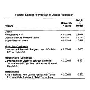
[0010] For example, in an embodiment, a predictive model is provided predicts
a risk
of prostate cancer progression in a patient, where the model is based on one
or more (e.g.,
all) of the features listed in Figure 11 and optionally other features. For
example, the
predictive model may be based on features including one or more (e.g., all) of
preoperative PSA, dominant Gleason Grade, Gleason Score, at least one of a
measurement of expression of AR in epithelial and/or stromal nuclei (e.g.,
tumor
epithelial and/or stromal nuclei) and a measurement of expression of Ki67-
positive
epithelial nuclei (e.g., tumor epithelial nuclei), a morphometric measurement
of average
edge length in the minimum spanning tree (MST) of epithelial nuclei, and a
morphometric measurement of area of non-lumen associated epithelial cells
relative to
total tumor area. In some embodiments, the dominant Gleason Grade comprises a
dominant biopsy Gleason Grade. In some embodiments, the Gleason Score
comprises a
biopsy Gleason Score.
[0011] In some embodiments of the present invention, two or more features
(e.g.,
clinical, molecular, and/or morphometric features) may be combined in order to
construct
a combined feature for evaluation within a predictive model. For example, in
the
embodiment of a predictive model predictive of prostate cancer progression
described
above, the measurement of the expression of androgen receptor (AR) in nuclei
(e.g.,
epithelial and/or stromal nuclei) may form a combined feature with the
measurement of
the expression of Ki67-positive epithelial nuclei. When a dominant Gleason
Grade for
the patient is less than or equal to 3, the predictive model may evaluate for
the combined
feature the measurement of the expression of androgen receptor (AR) in
epithelial and
stromal nuclei. Conversely, when the dominant Gleason Grade for the patient is
4 or 5,
the predictive model may evaluate for the combined feature the measurement of
the
expression of Ki67-positive epithelial nuclei.
[0012] Additional examples of combined features according to some embodiments
of
the present invention are described below in connection with, for example,
Figure 9. For
4
CA 3074969 2020-03-09
example, in the embodiment of a predictive model predictive of prostate cancer
progression described above, the morphometric measurement of average edge
length in
the minimum spanning tree (MST) of epithelial nuclei may form a combined
feature with
dominant Gleason Grade. When the dominant Gleason Grade for the patient is
less than
or equal to 3, the predictive model may evaluate for the combined feature the
measurement of average edge length in the minimum spanning tree (MST) of
epithelial
nuclei. Conversely, when the dominant Gleason Grade for the patient is 4 or 5,
the
predictive model may evaluate the dominant Gleason Grade for the combined
feature.
[0013] In some embodiments of the present invention, a model is provided which
is
predictive of an outcome with respect to a medical condition (e.g., presence,
recurrence,
or progression of the medical condition), where the model is based on one or
more
computer-generated morphometric features generated from one or more images of
tissue
subject to multiplex immunofluorescence (IF). For example, due to highly
specific
identification of molecular components and consequent accurate delineation of
tissue
compartments attendant to multiplex IF (e.g., as compared to the stains used
in light
microscopy), multiplex IF microscopy may provide the advantage of more
reliable and
accurate image segmentation. The model may be configured to receive a patient
dataset
for the patient, and evaluate the patient dataset according to the model to
produce a value
indicative of the patient's risk of occurrence of the outcome. In some
embodiments, the
predictive model may also be based on one or more other morphometric features,
one or
more clinical features, and/or one or more molecular features.
[0014] For example, in some embodiments of the present invention, the
predictive
model may be based on one or more computer-generated morphometric feature(s)
including one or more measurements of the minimum spanning tree (MST) (e.g.,
the
MST of epithelial nuclei) identified in the one or more images of tissue
subject to
multiplex immunofluorescence (IF). For example, the one or more measurements
of the
minimum spanning tree (MST) may include the average edge length in the MST of
epithelial nuclei. Other measurements of the MST according to some embodiments
of
the present invention are described below in connection with, for example,
Figure 9.
[0015] In some embodiments of the present invention, the predictive model may
be
based on one or more computer-generated morphometric feature(s) including one
or more
CA 3074969 2020-03-09
measurements of the fractal dimension (FD) (e.g., the FD of one or more
glands)
measured in the one or more images of tissue subject to multiplex
immunofluorescence
(IF). For example, the one or more measurements of the fractal dimension (FD)
may
include one or more measurements of the fractal dimension of gland boundaries
between
glands and stroma. In another example, the one or more measurements of the
fractal
dimension (FD) may include one or more measurements of the fractal dimension
of gland
boundaries between glands and stroma and between glands and lumen.
[0016] In an aspect of embodiments of the present invention, systems and
methods are
provided for segmenting and classifying objects in images of tissue subject to
multiplex
immunofluorescence (IF). For example, such segmentation and classification may
include initial segmentation into primitives, classification of primitives
into nuclei,
cytoplasm, and background, and refinement of the classified primitives to
obtain the final
segmentation, in the manner described below in connection with Figure 6.
[0017] In some embodiments, an apparatus is provided for identifying objects
of
interest in images of tissue, where the apparatus includes an image analysis
tool
configured to segment a tissue image into pathological objects comprising
glands.
Starting with lumens in the tissue image identified as seeds, the image
analysis tool is
configured to perform controlled region growing on the image including
initiating growth
around the lumen seeds in the tissue image thus encompassing epithelial cells
identified
in the image through the growth. The image analysis tool continues growth of
each gland
around each lumen seed so long as the area of each successive growth ring is
larger than
the area of the preceding growth ring. The image analysis tool discontinues
the growth of
the gland when the area of a growth ring is less than the area of the
preceding growth ring
for the gland.
[0018] In some embodiments, an apparatus is provided for measuring the
expression of
one or more biomarkers in images of tissue subject to immunofluorescence (IF),
where
the apparatus includes an image analysis tool configured to measure within an
IF image
of tissue the intensity of a biomarker (e.g., AR) as expressed within a
particular type of
pathological object (e.g., epithelial nuclei). Specifically, a plurality of
percentiles of the
intensity of the biomarker as expressed within the particular type of
pathological object
are determined. The image analysis tool identifies one of the plurality of
percentiles as
6
CA 3074969 2020-03-09
the percentile corresponding to a positive level of the biomarker in the
pathological
object. For example, the image analysis tool may identify the percentile
correspond to a
positive level of the biomarker based at least in part on an intensity in a
percentile of
another pathological object (e.g., stroma nuclei). In some embodiments, the
image
analysis tool is further configured to measure one or more features from the
image of
tissue, wherein the one or more features includes a difference of intensities
of the
percentile values (e.g., percentiles 90 and 10 of AR in epithelial nuclei).
For example,
the one or more features may include a difference of intensities of the
percentile values
normalized by an image threshold or another difference in intensities of
percentile values
(e.g., percentiles 90 and 10 in stroma nuclei).
10019] In some embodiments, an apparatus is provided for identifying objects
of
interest in images of tissue, where the apparatus includes an image analysis
tool
configured to detect the presence of CD34 in an image of tissue subject to
immunofluorescence (IF). Based on the detection, the image analysis tool is
further
configured to detect and segment blood vessels which are in proximity to the
CD34.
100201 In another aspect of embodiments of the present invention, systems and
methods
are provided in which data for a patient is measured at each of a plurality of
points in
time and evaluated by a predictive model of the present invention. A diagnosis
or
treatment of the patient may be based on a comparison of the results from each
evaluation. Such a comparison may be summarized in, for example, a report
output by a
computer for use by a physician or other individual. For example, systems and
methods
may be provided for screening for an inhibitor compound of a medical
condition. A first
dataset for a patient may be evaluated by a predictive model, where the model
is based on
clinical data, molecular data, and computer-generated morphometric data. A
test
compound may be administered to the patient. Following administering of the
test
compound, a second dataset may be obtained from the patient and evaluated by
the
predictive model. The results of the evaluation of the first dataset may be
compared to
the results of the evaluation from the second dataset. A change in the results
for the
second dataset with respect to the first dataset may indicate that the test
compound is an
inhibitor compound.
7
CA 3074969 2020-03-09
[0021] In still another aspect of embodiments of the present invention, a test
kit is
provided for treating, diagnosing and/or predicting the occurrence of a
medical condition.
Such a test kit may be situated in a hospital, other medical facility, or any
other suitable
location. The test kit may receive data for a patient (e.g., including
clinical data,
molecular data, and/or computer-generated morphometric data), compare the
patient's
data to a predictive model (e.g., programmed in memory of the test kit) and
output the
results of the comparison. In some embodiments, the molecular data and/or the
computer-generated morphometric data may be at least partially generated by
the test kit.
For example, the molecular data may be generated by an analytical approach
subsequent
to receipt of a tissue sample for a patient. The morphometric data may be
generated by
segmenting an electronic image of the tissue sample into one or more objects,
classifying
the one or more objects into one or more object classes (e.g., epithelial
nuclei, epithelial
cytoplasm, stroma, lumen, red blood cells, etc.), and determining the
morphometric data
by taking one or more measurements for the one or more object classes. In some
embodiments, the test kit may include an input for receiving, for example,
updates to the
predictive model. In some embodiments, the test kit may include an output for,
for
example, transmitting data, such as data useful for patient billing and/or
tracking of
usage, to another device or location.
BRIEF DESCRIPTION OF THE DRAWINGS
[0022] For a better understanding of embodiments of the present invention,
reference is
made to the following detailed description, taken in conjunction with the
accompanying
drawings, in which like reference characters refer to like parts throughout,
and in which:
[0023] Figures IA and 1B are block diagrams of systems that use a predictive
model to
treat, diagnose or predict the occurrence of a medical condition according to
some
embodiments of the present invention;
[0024] Figure IC is a block diagram of a system for generating a predictive
model
according to some embodiments of the present invention;
[0025] Figure 2 is a graph illustrating the probability that a patient will
experience an
outcome with respect to a medical condition (e.g., disease progression) as
indicated by
the value or score output by a predictive model according to some embodiments
of the
present invention;
8
CA 3074969 2020-03-09
[0026] Figure 3 is a flowchart of illustrative stages involved in image
segmentation and
object classification in, for example, digitized images of H&E-stained tissue
according to
some embodiments of the present invention;
[0027] Figure 4A is an image of prostate tissue obtained via a needle biopsy
and subject
to staining with hernatoxylin and eosin (H&E) according to some embodiments of
the
present invention;
[0028] Figure 4B is a segmented and classified version of the image in Figure
4A
according to some embodiments of the present invention, in which gland unit
objects are
formed from seed lumen, epithelial nuclei, and epithelial cytoplasm, and in
which
isolated/non¨gland-associated tumor epithelial cells are also identified in
the image;
[0029] Figure 5A is an image of tissue subject to multiplex immunofluorescence
(IF) in
accordance with some embodiments of the present invention;
[0030] Figure 5B shows a segmented and classified version of the image in
Figure 4A,
in which the objects epithelial nuclei, cytoplasm, and stroma nuclei have been
identified
according to some embodiments of the present invention;
[0031] Figure 6 is a flowchart of illustrative stages involved in image
segmentation and
object classification in images of tissue subject to multiplex
immunofluorescence (IF)
according to some embodiments of the present invention;
[0032] Figure 7 is a flowchart of illustrative stages involved in constructing
the
minimum spanning tree (MST) of objects within an image of tissue subject to
multiplex
immunofluorescence (IF) according to some embodiments of the present
invention;
[0033] Figure 8A is an image of tissue subject to multiplex immunofluorescence
(IF) in
which the minimum spanning tree (MST) of epithelial nuclei (EN) is identified
in
accordance with some embodiments of the present invention;
[0034] Figure 8B is an image of tissue subject to multiplex immunofluorescence
(IF) in
which the boundaries of glands with stroma and the boundaries of glands with
lumen are
identified according to some embodiments of the present invention;
[0035] Figure 9 is a listing of minimum spanning tree (MST) features, fractal
dimension (FD) features, combined features, and their respective two-sided p-
values and
values of the concordance index, which were identified in images of tissue
subject to
9
CA 3074969 2020-03-09
multiplex immunofluorescence (IF) and which may be used in predictive models
according to some embodiments of the present invention;
[0036] Figure 10 is a flowchart of illustrative stages involved in screening
for an
inhibitor compound in accordance with an embodiment of the present invention;
[0037] Figure 11 is a listing of clinical, molecular, and computer-generated
morphometric features used by a model to predict disease progression in a
patient
according to an embodiment of the present invention;
[0038] Figure 12 are Kaplan-Meier curves illustrating the ability of a feature
used in the
predictive model of Figure 11 to accurately stratify patients into low and
high risk
groups, namely the morphometric feature of area of isolated (non-lumen
associated)
tumor epithelial cells relative to total tumor area;
[0039] Figure 13 is a graph of a Kaplan-Meier curve illustrating the ability
of another
feature used in the predictive model of Figure 11 to accurately stratify
patients into low
and high risk groups, namely the morphometric feature of mean edge length in
the
minimum spanning tree (MST) of all edges connecting epithelial nuclei
centroids (for
dominant biopsy Gleason grade (bGG) < 3) in combination with the clinical
feature of
Gleason grade (for bGG = 4 or 5);
[0040] Figure 14 is a graph of a Kaplan-Meier curve illustrating the ability
of yet
another feature used in the predictive model of Figure 11 to accurately
stratify patients
into low and high risk groups, namely the molecular feature of AR dynamic
range (for
bGG < 3) in combination with the molecular feature of total Ki67 (for bGG = 4
or 5);
[0041] Figure 15 is a graph of a Kaplan-Meier curve illustrating the ability
of the value
or score output by the predictive model of Figure 11 to stratify patients in
the training set
according to risk; and
[0042] Figure 16 is a graph of a Kaplan-Meier curve illustrating the ability
of the value
or score output by the predictive model of Figure 11 to stratify patients in
the validation
set according to risk.
DETAILED DESCRIPTION OF THE INVENTION
[0043] Embodiments of the present invention relate to methods and systems that
use
computer-generated morphometric information, clinical information, and/or
molecular
information in a predictive model for predicting the occurrence of a medical
condition.
CA 3074969 2020-03-09
For example, in some embodiments of the present invention, clinical, molecular
and
computer-generated morphometric information are used to predict the likelihood
or risk
of progression of a disease such as, for example, prostate cancer. In other
embodiments,
the teachings provided herein are used to predict the occurrence (e.g.,
presence,
recurrence, or progression) of other medical conditions such as, for example,
other types
of disease (e.g., epithelial and mixed-neoplasms including breast, colon,
lung, bladder,
liver, pancreas, renal cell, and soft tissue) and the responsiveness or
unresponsiveness of
a patient to one or more therapies (e.g., pharmaceutical drugs). These
predictions may be
used by physicians or other individuals, for example, to select an appropriate
course of
treatment for a patient, diagnose a medical condition in the patient, and/or
predict the risk
or likelihood of disease progression in the patient.
100441 In an aspect of the present invention, an analytical tool such as, for
example, a
module configured to perform support vector regression for censored data
(SVRc), a
support vector machine (SVM), and/or a neural network may be provided that
determines
correlations between clinical features, molecular features, computer-generated
morphometric features, combinations of such features, and/or other features
and a
medical condition. The correlated features may form a model that can be used
to predict
an outcome with respect to the condition (e.g., presence, recurrence, or
progression). For
example, an analytical tool may be used to generate a predictive model based
on data for
a cohort of patients whose outcomes with respect to a medical condition (e.g.,
time to
recurrence or progression of cancer) are at least partially known. The model
may then be
used to evaluate data for a new patient in order to predict the risk of
occurrence of the
medical condition in the new patient. In some embodiments, only a subset of
clinical,
molecular, morphometric, and/or other data (e.g., clinical and morphometric
data only)
may be used by the analytical tool to generate the predictive model.
Illustrative systems
and methods for treating, diagnosing, and predicting the occurrence of medical
conditions
are described in commonly-owned U.S. Patent No. 7,461,048, issued December
2,2008,
U.S. Patent No. 7,467,119, issued December 16, 2008, and PCT published
Application
No. WO 2008/124138, published October 16, 2008.
II
CA 3074969 2020-03-09
[0045] The clinical, molecular, and/or morphometric data used by embodiments
of the
present invention may include any clinical, molecular, and/or morphometric
data that is
relevant to the diagnosis, treatment and/or prediction of a medical condition.
For
example, features analyzed for correlations with progression of prostate
cancer in order to
generate a model predictive of prostate cancer progression are described below
in
connection with Tables 1-5 and 9 and Figure 9. It will be understood that at
least some of
these features (e.g., epithelial and mixed-neoplasms) may provide a basis for
developing
predictive models for other medical conditions (e.g., breast, colon, lung,
bladder, liver,
pancreas, renal cell, and soft tissue). For example, one or more of the
features in Tables
1-5 and 9 and Figure 9 may be assessed for patients having some other medical
condition
and then input to an analytical tool that determines whether the features
correlate with the
medical condition. Generally, features that increase the ability of the model
to predict the
occurrence of the medical condition (e.g., as determined through suitable
univariate
and/or multivariate analyses) may be included in the final model, whereas
features that do
not increase (e.g., or decrease) the predictive power of the model may be
removed from
consideration. By way of example only, illustrative systems and methods for
selecting
features for use in a predictive model are described below and in commonly-
owned U.S.
Publication No. 2007/0112716, published May 17, 2007 and entitled "Methods and
Systems for Feature Selection in Machine Learning Based on Feature
Contribution and
Model Fitness''.
100461 Using the features in Tables 1-5 and 9 and Figure 9 as a basis for
developing a
predictive model may focus the resources of physicians, other individuals,
and/or
automated processing equipment (e.g., a tissue image analysis system) on
obtaining
patient data that is more likely to be correlated with outcome and therefore
useful in the
final predictive model. Moreover, the features determined to be correlated
with
progression of prostate cancer are shown in Table 9 and Figure 11 . It will be
understood
that these features may be included directly in final models predictive of
progression of
prostate cancer and/or used for developing predictive models for other medical
conditions.
100471 The morphometric data used in predictive models according to some
embodiments of the present invention may include computer-generated data
indicating
12
CA 3074969 2020-03-09
various structural, textural, and/or spectral properties of, for example,
tissue specimens.
For example, the morphometric data may include data for morphometric features
of
stroma, cytoplasm, epithelial nuclei, stroma nuclei, lumen, red blood cells,
tissue
artifacts, tissue background, glands, other objects identified in a tissue
specimen or a
digitized image of such tissue, or a combination thereof.
100481 In an aspect of the present invention, a tissue image analysis system
is provided
for measuring morphometric features from tissue specimen(s) (e.g., needle
biopsies
and/or whole tissue cores) or digitized image(s) thereof. The system may
utilize, in part,
the commercially-available Definiens Cellenger software. For example, in some
embodiments, the image analysis system may receive image(s) of tissue stained
with
hematoxylin and eosin (H&E) as input, and may output one or more measurements
of
morphometric features for pathological objects (e.g., epithelial nuclei,
cytoplasm, etc.)
and/or structural, textural, and/or spectral properties observed in the
image(s). For
example, such an image analysis system may include a light microscope that
captures
images of H&E-stained tissue at 20X magnification. Illustrative systems and
methods for
measuring morphometric features from images of H&E-stained tissue according to
some
embodiments of the present invention are described below in connection with,
for
example, Figure 3 and the illustrative study in which aspects of the present
invention
were applied to prediction of prostate cancer progression. Computer-generated
morphometric features (e.g., morphometric features measurable from digitized
images of
H&E-stained tissue) which may be used in a predictive model for predicting an
outcome
with respect to a medical condition according to some embodiments of the
present
invention are summarized in Table I.
100491 In some embodiments of the present invention, the image analysis system
may
receive image(s) of tissue subject to multiplex immunofluoreseence (IF) as
input, and
may output one or more measurements of morphometric features for pathological
objects
(e.g., epithelial nuclei, cytoplasm, etc.) and/or structural, textural, and/or
spectral
properties observed in the image(s). For example, such an image analysis
system may
include a multispectral camera attached to a microscope that captures images
of tissue
under an excitation light source. Computer-generated morphometric features
(e.g.,
morphometric features measurable from digitized images of tissue subject to
multiplex
13
CA 3074969 2020-03-09
IF) which may be used in a predictive model for predicting an outcome with
respect to a
medical condition according to some embodiments of the present invention are
listed in
Table 2. Illustrative examples of such morphometric features include
characteristics of a
minimum spanning tree (MST) (e.g., MST connecting epithelial nuclei) and/or a
fractal
dimension (FD) (e.g., FD of gland boundaries) measured in images acquired
through
multiplex IF microscopy. Illustrative systems and methods for measuring
morphometric
features from images of tissue subject to multiplex IF according to some
embodiments of
the present invention are described below in connection with, for example,
Figures 4B-9
and the illustrative study in which aspects of the present invention were
applied to the
prediction of prostate cancer progression.
10050] Clinical features which may be used in predictive models according to
some
embodiments of the present invention may include or be based on data for one
or more
patients such as age, race, weight, height, medical history, genotype and
disease state,
where disease state refers to clinical and pathologic staging characteristics
and any other
clinical features gathered specifically for the disease process under
consideration.
Generally, clinical data is gathered by a physician during the course of
examining a
patient and/or the tissue or cells of the patient. The clinical data may also
include clinical
data that may be more specific to a particular medical context. For example,
in the
context of prostate cancer, the clinical data may include data indicating
blood
concentration of prostate specific antigen (PSA), the result of a digital
rectal exam,
Gleason score, and/or other clinical data that may be more specific to
prostate cancer.
Clinical features which may be used in a predictive model for predicting an
outcome with
respect to a medical condition according to some embodiments of the present
invention
are listed in Table 3.
[00511 Molecular features which may be used in predictive models according to
some
embodiments of the present invention may include or be based on data
indicating the
presence, absence, relative increase or decrease or relative location of
biological
molecules including nucleic acids, polypeptides, saccharides, steroids and
other small
molecules or combinations of the above, for example, glycoroteins and protein-
RNA
complexes. The locations at which these molecules are measured may include
glands,
tumors, stroma, and/or other locations, and may depend on the particular
medical context.
14
CA 3074969 2020-03-09
Generally, molecular data is gathered using molecular biological and
biochemical
techniques including Southern, Western, and Northern blots, polymerase chain
reaction
(PCR), immunohistochemistry, and/or immunofluorescence (IF) (e.g., multiplex
IF).
Molecular features which may be used in a predictive model for predicting an
outcome
with respect to a medical condition according to some embodiments of the
present
invention are listed in Table 4. Additional details regarding multiplex
immunofluorescence according to some embodiments of the present invention are
described in commonly-owned U.S. Patent Application Publication No.
2007/0154958,
published July 5, 2007 and entitled "Multiplex In Situ Immunohistochernical
Analysis ".
Further, in situ
hybridization may be used to show both the relative abundance and location of
molecular
biological features. Illustrative methods and systems for in situ
hybridization of tissue
are described in, for example, commonly-owned U.S. Patent No. 6,995,020,
issued
February 7, 2006 and entitled "Methods and compositions for the preparation
and use of
fixed-treated cell-lines and tissue in fluorescence in situ hybridization
100521 Generally, when any clinical, molecular, and/or morphometric features
from any
of Tables 1-5 and 9 and/or Figures 9 and 11 are applied to medical contexts
other than the
prostate, features from these Tables and/or Figures that are more specific to
the prostate
may not be considered. Optionally, features more specific to the medical
context in
question may be substituted for the prostate-specific features. For example,
other
histologic disease-specific features/manifestations may include regions of
necrosis (e.g.,
ductal carcinoma in situ for the breast), size, shape and regional
pattern/distribution of
epithelial cells (e.g., breast, lung), degree of differentiation (e.g.,
squamous
differentiation with non-small cell lung cancer (NSCLC, mucin production as
seen with
various adenocarcinomas seen in both breast and colon)),
morphological/microscopic
distribution of the cells (e.g., lining ducts in breast cancer, lining
bronchioles in NSCLC),
and degree and type of inflammation (e.g., having different characteristics
for breast and
NSCLC in comparison to prostate).
[0053] Figures IA and 1B show illustrative systems that use a predictive model
to
predict the occurrence (e.g., presence, recurrence, or progression) of a
medical condition
CA 3074969 2020-03-09
in a patient. The arrangement in Figure IA may be used when, for example, a
medical
diagnostics lab provides support for a medical decision to a physician or
other individual
associated with a remote access device. The arrangement in Figure 1B may be
used
when, for example, a test kit including the predictive model is provided for
use in a
facility such as a hospital, other medical facility, or other suitable
location.
[0054] Referring to Figure 1A, predictive model 102 is located in diagnostics
facility 104. Predictive model 102 may include any suitable hardware,
software, or
combination thereof for receiving data for a patient, evaluating the data in
order to predict
the occurrence (e.g., presence, recurrence, or progression) of a medical
condition for the
patient, and outputting the results of the evaluation. In another embodiment,
model 102
may be used to predict the responsiveness of a patient to particular one or
more therapies.
Diagnostics facility 104 may receive data for a patient from remote access
device 106 via
Internet service provider (1SP) 108 and communications networks 110 and 112,
and may
input the data to predictive model 102 for evaluation. Other arrangements for
receiving
and evaluating data for a patient from a remote location are of course
possible (e.g., via
another connection such as a telephone line or through the physical mail). The
remotely
located physician or individual may acquire the data for the patient in any
suitable
manner and may use remote access device 106 to transmit the data to
diagnostics
facility 104. In some embodiments, the data for the patient may be at least
partially
generated by diagnostics facility 104 or another facility. For example,
diagnostics facility
104 may receive a digitized image of H&E-stained tissue from remote access
device 106
or other device and may generate morphometric data for the patient based on
the image.
In another example, actual tissue samples may be received and processed by
diagnostics
facility 104 in order to generate morphometric data, molecular data, and/or
other data. In
other examples, a third party may receive a tissue sample or image for a new
patient,
generate morphometric data, molecular data and/or other data based on the
image or
tissue, and provide the morphometric data, molecular data and/or other data to
diagnostics facility 104. Illustrative embodiments of suitable image
processing tools for
generating morphometric data and/or molecular data from tissue images and/or
tissue
samples according to some embodiments of the present invention are described
below in
connection with Figures 3-8.
16
CA 3074969 2020-03-09
[0055] Diagnostics facility 104 may provide the results of the evaluation to a
physician
or individual associated with remote access device 106 through, for example, a
transmission to remote access device 106 via ISP 108 and communications
networks 110
and 112 or in another manner such as the physical mail or a telephone call.
The results
may include a value or "score" (e.g., an indication of the likelihood that the
patient will
experience one or more outcomes related to the medical condition such as the
presence of
the medical condition, predicted time to recurrence of the medical condition,
or risk or
likelihood of progression of the medical condition in the patient),
information indicating
one or more features analyzed by predictive model 102 as being correlated with
the
medical condition, image(s) output by the image processing tool, information
indicating
the sensitivity and/or specificity of the predictive model, explanatory
remarks, other
suitable information, or a combination thereof. For example, Figure 2 shows at
least a
portion of a report for a fictional patient that may be output by, or
otherwise generated
based on the output of, the predictive model. As shown, the report may
indicate that
based on the data for the patient input to the predictive model, the
predictive model
output a value of 40 corresponding to a 19% probability of disease progression
(as
indicated by castrate PSA rise, metastasis and/or prostate cancer mortality)
within eight
years after radical prostatectomy, which may place the patient in a high-risk
category.
(Conversely, as indicated by the vertical line in the embodiment shown in
Figure 2, a
values of less than 30.19 output by the predictive model may place the patient
in a low-
risk category.) Such a report may be used by a physician or other individual,
for
example, to assist in determining appropriate treatment option(s) for the
patient. The
report may also be useful in that it may help the physician or individual to
explain the
patient's risk to the patient.
100561 Remote access device 106 may be any remote device capable of
transmitting
and/or receiving data from diagnostics facility 104 such as, for example, a
personal
computer, a wireless device such as a laptop computer, a cell phone or a
personal digital
assistant (PDA), or any other suitable remote access device. Multiple remote
access
devices 106 may be included in the system of Figure lA (e.g., to allow a
plurality of
physicians or other individuals at a corresponding plurality of remote
locations to
communicate data with diagnostics facility 104), although only one remote
access device
17
CA 3074969 2020-03-09
106 has been included in Figure lA to avoid over-complicating the drawing.
Diagnostics
facility 104 may include a server capable of receiving and processing
communications to
and/or from remote access device 106. Such a server may include a distinct
component
of computing hardware and/or storage, but may also be a software application
or a
combination of hardware and software. The server may be implemented using one
or
more computers.
100571 Each of communications links 110 and 112 may be any suitable wired or
wireless communications path or combination of paths such as, for example, a
local area
network, wide area network, telephone network, cable television network,
intranet, or
Internet. Some suitable wireless communications networks may be a global
system for
mobile communications (GSM) network, a time-division multiple access (TDMA)
network, a code-division multiple access (CDMA) network, a Bluetooth network,
or any
other suitable wireless network.
[0058] Figure 1B shows a system in which test kit 122 including a predictive
model in
accordance with an embodiment of the present invention is provided for use in
facility
124, which may be a hospital, a physician's office, or other suitable
location. Test kit
122 may include any suitable hardware, software, or combination thereof (e.g.,
a personal
computer) that is adapted to receive data for a patient (e.g., at least one of
clinical,
morphometric and molecular data), evaluate the patient's data with a
predictive model
(e.g., programmed in memory of the test kit), and output the results of the
evaluation.
For example, test kit 122 may include a computer readable medium encoded with
computer executable instructions for performing the functions of the
predictive model.
The predictive model may be a predetermined model previously generated (e.g.,
by
another system or application such as the system in Figure 1C). In some
embodiments,
test kit 122 may optionally include an image processing tool capable of
generating data
corresponding to morphometric and/or molecular features from, for example, a
tissue
sample or image. Illustrative embodiments of suitable image processing tools
according
to some embodiments of the present invention are described below in connection
with
Figures 3-8. In other embodiments, test kit 122 may receive pre-packaged data
for the
morphometric features as input from, for example, an input device (e.g.,
keyboard) or
another device or location. Test kit 122 may optionally include an input for
receiving, for
18
CA 3074969 2020-03-09
example, updates to the predictive model. The test kit may also optionally
include an
output for transmitting data, such as data useful for patient billing and/or
tracking of
usage, to a main facility or other suitable device or location. The billing
data may
include, for example, medical insurance information for a patient evaluated by
the test kit
(e.g., name, insurance provider, and account number). Such information may be
useful
when, for example, a provider of the test kit charges for the kit on a per-use
basis and/or
when the provider needs patients' insurance information to submit claims to
insurance
providers.
[00591 Figure IC shows an illustrative system for generating a predictive
model. The
system includes analytical tool 132 (e.g., including a module configured to
perform
support vector regression for censored data (SVRc), a support vector machine
(SVM),
and/or a neural network) and database 134 of patients whose outcomes are at
least
partially known. Analytical tool 132 may include any suitable hardware,
software, or
combination thereof for determining correlations between the data from
database 134 and
a medical condition. The system in Figure 1C may also include image processing
tool
136 capable of generating, for example, morphometric data based on H&E-stained
tissue
or digitized image(s) thereof, morphometric data and/or molecular data based
on tissue
acquired using multiplex immunofluorescence (IF) microscopy or digitized
image(s) of
such tissue, or a combination thereof. Tool 136 may generate morphometric data
and/or
molecular data for, for example, the known patients whose data is included in
database
134. Illustrative embodiments of suitable image processing tools according to
some
embodiments of the present invention are described below in connection with
Figures 3-
8.
[0060] Database 134 may include any suitable patient data such as data for
clinical
features, morphometric features, molecular features, or a combination thereof.
Database
134 may also include data indicating the outcomes of patients such as whether
and when
the patients have experienced a disease or its recurrence or progression. For
example,
database 134 may include uncensored data for patients (i.e., data for patients
whose
outcomes are completely known) such as data for patients who have experienced
a
medical condition or its recurrence or progression. Database 134 may
alternatively or
additionally include censored data for patients (i.e., data for patients whose
outcomes are
19
CA 3074969 2020-03-09
not completely known) such as data for patients who have not shown signs of a
disease or
its recurrence or progression in one or more follow-up visits to a physician.
The use of
censored data by analytical tool 132 may increase the amount of data available
to
generate the predictive model and, therefore, may advantageously improve the
reliability
and predictive power of the model. Examples of machine learning approaches,
namely
support vector regression for censored data (SVRc) and a particular
implementation of a
neural network (NNci) that can make use of both censored and uncensored data
are
described below.
100611 In one embodiment, analytical tool 132 may perform support vector
regression
on censored data (SVRc) in the manner set forth in commonly-owned U.S. Patent
No.
7,505,948, issued March 17, 2009.
SVRc uses a loss/penalty function which is modified relative to support vector
machines (SVM) in order to allow for the utilization of censored data. For
example, data
including clinical, molecular, and/or morphometric features of known patients
from
database 134 may be input to the SVRc to determine parameters for a predictive
model.
The parameters may indicate the relative importance of input features, and may
be
adjusted in order to maximize the ability of the SVRc to predict the outcomes
of the
known patients.
[0062] The use of SVRc by analytical tool 132 may include obtaining from
database
134 multi-dimensional, non-linear vectors of information indicative of status
of patients,
where at least one of the vectors lacks an indication of a time of occurrence
of an event or
outcome with respect to a corresponding patient. Analytical tool 132 may then
perform
regression using the vectors to produce a kernel-based model that provides an
output
value related to a prediction of time to the event based upon at least some of
the
information contained in the vectors of information. Analytical tool 132 may
use a loss
function for each vector containing censored data that is different from a
loss function
used by tool 132 for vectors comprising uncensored data. A censored data
sample may
be handled differently because it may provide only "one-sided information."
For
example, in the case of survival time prediction, a censored data sample
typically only
indicates that the event has not happened within a given time, and there is no
indication
of when it will happen after the given time, if at all.
CA 3074969 2020-03-09
[0063] The loss function used by analytical tool 132 for censored data may be
as
follows:
{C; (e ¨ e's) e >
Loss( f (x),y,s = 1) = 0 ¨Es <e<E:,
C s(e s¨e) e<¨e,
where e = f (x)¨ y ; and
f (x) = WT (x) + b
is a linear regression function on a feature space F. Here, W is a vector in
F, and 436(x)
maps the input x to a vector in F.
[0064] In contrast, the loss function used by tool 132 for uncensored data may
be:
{Cõ (e ¨ e) .. e >
Loss( f (x), y,s =0) = 0 n < e < e,, ,
C õ(E ¨ e) e < ¨E
where e = f(x)¨ y
and E õ and Cõ Cõ
[0065] In the above description, the W and b are obtained by solving an
optimization
problem, the general form of which is:
min ¨1 W' W
W, b 2
s.t. Y, ¨ (WTO(x,)+ b)
(Wr Axi)+b) ¨ 5- e
This equation, however, assumes the convex optimization problem is always
feasible,
which may not be the case. Furthermore, it is desired to allow for small
errors in the
regression estimation. It is for these reasons that a loss function is used
for SVRc. The
loss allows some leeway for the regression estimation. Ideally, the model
built will
exactly compute all results accurately, which is infeasible. The loss function
allows for a
range of error from the ideal, with this range being controlled by slack
variables and e,
and a penalty C. Errors that deviate from the ideal, but are within the range
defined by
21
CA 3074969 2020-03-09
and (,are counted, but their contribution is mitigated by C. The more
erroneous the
instance, the greater the penalty. The less erroneous (closer to the ideal)
the instance is,
the less the penalty. This concept of increasing penalty with error results in
a slope, and
C controls this slope. While various loss functions may be used, for an
epsilon-
insensitive loss function, the general equation transforms into:
I T
min
W,b 2
si.
(WT (1)(;)+b) Y , e
0, i =1. = = 1
For an epsilon-insensitive loss function in accordance with the invention
(with different
loss functions applied to censored and uncensored data), this equation
becomes:
min Pe
W,b 2
st. y, ¨(WT(13(x1)+b) e,
(WrcD(x,)+ b)¨ y,
> 0, i =1. = =
where C'') = s,Cr) + (1¨ s,)Cõ(')
= s,er) + (1¨ s, )e
[0066] The optimization criterion penalizes data points whose y-values differ
from f(x)
by more than e. The slack variables, 4 and correspond to the size of this
excess
deviation for positive and negative deviations respectively. This penalty
mechanism has
two components, one for uncensored data (i.e., not right-censored) and one for
censored
data. Here, both components are represented in the form of loss functions that
are
referred to as a-insensitive loss functions.
100671 In another embodiment, analytical tool 132 may include a neural
network. In
such an embodiment, tool 132 preferably includes a neural network that is
capable of
utilizing censored data. Additionally, the neural network preferably uses an
objective
function substantially in accordance with an approximation (e.g., derivative)
of the
concordance index (Cl) to train an associated model (NNei). Though the CI has
long
been used as a performance indicator for survival analysis [12], the use of
the CI to train
22
CA 3074969 2020-03-09
a neural network was proposed in commonly-owned U.S. Patent No. 7,321,881,
issued
January 22, 2008. The
difficulty of using the Cl as a training objective function in the past is
that the Cl is non-
differentiable and cannot be optimized by gradient-based methods. As described
in
U.S. Patent No. 7,321,881, this obstacle may be overcome by using
an approximation of the CI as the objective function.
[0068] For example, when analytical tool 132 includes a neural network that is
used to
predict prostate cancer progression, the neural network may process input data
for a
cohort of patients whose outcomes with respect to prostate cancer progression
are at least
partially known in order to produce an output. The particular features
selected for input
to the neural network may be selected through the use of the above-described
SVRc (e.g.,
implemented with analytical tool 132) or any other suitable feature selection
process. An
error module of tool 132 may determine an error between the output and a
desired output
corresponding to the input data (e.g., the difference between a predicted
outcome and the
known outcome for a patient). Analytical tool 132 may then use an objective
function
substantially in accordance with an approximation of the Cl to rate the
performance of
the neural network. Analytical tool 132 may adapt the weighted connections
(e.g.,
relative importance of features) of the neural network based upon the results
of the
objective function.
[0069] The concordance index may be expressed in the form:
y 16,1j)
= __________________________________________
lI
where
>1
0:otherwise
and may be based on pair-wise comparisons between the prognostic estimates i
and
i, for patients i and j, respectively. In this example, consists of all the
pairs of patients
(i,j) who meet the following conditions:
23
CA 3074969 2020-03-09
= both patients i and j experienced recurrence, arid the recurrence
time t, of patient i is shorter than patient j's recurrence time tj; or
= only patient i experienced recurrence and 1, is shorter than patient j's
follow-up visit time
The numerator of the CI represents the number of times that the patient
predicted to recur
earlier by the neural network actually does recur earlier. The denominator is
the total
number of pairs of patients who meet the predetermined conditions.
[0070] Generally, when the CI is increased, preferably maximized, the model is
more
accurate. Thus, by preferably substantially maximizing the Cl, or an
approximation of
the CI, the performance of a model is improved. In accordance with some
embodiments
of the present invention, an approximation of the Cl is provided as follows:
R(i I )
c =Zo.paz
II
where
R(i,,i,)= (¨(1, ¨r)Y1 <Y1
0: otherwise
and where 0 <y < I and n> 1. R(i,,Iõ) can be regarded as an approximation to
[0071] Another approximation of the CI provided in accordance with some
embodiments of the present invention which has been shown empirically to
achieve
improved results is the following:
E Fa ¨ (1, ¨1,)= R(I,,11)
C'õ = ____________________________________________
where
24
CA 3074969 2020-03-09
D=
0.ixa
is a normalization factor. Here each is
weighted by the difference between i, and
if . The process of minimizing the Ca, (or C) seeks to move each pair of
samples in f2 to
satisfyi, > y and thus to make /(iõ )= 1.
[0072] When the difference between the outputs of a pair in SZ is larger than
the margin
y, this pair of samples will stop contributing to the objective function. This
mechanism
effectively overcomes over-fitting of the data during training of the model
and makes the
optimization preferably focus on only moving more pairs of samples in n to
satisfy
i, > y. The influence of the training samples is adaptively adjusted
according to the
pair-wise comparisons during training. Note that the positive margin y in R is
preferable
for improved generalization performance. In other words, the parameters of the
neural
network are adjusted during training by calculating the CI after all the
patient data has
been entered. The neural network then adjusts the parameters with the goal of
minimizing the objective function and thus maximizing the CI. As used above,
over-
fitting generally refers to the complexity of the neural network.
Specifically, if the
network is too complex, the network will react to "noisy" data. Overfitting is
risky in
that it can easily lead to predictions that are far beyond the range of the
training data.
[0073] Morphometric Data Obtained from H&E-Stained Tissue
[0074] As described above, an image processing tool (e.g., image processing
tool 136)
in accordance with some embodiments of the present invention may be provided
that
generates digitized images of tissue specimens (e.g., H&E-stained tissue
specimens)
and/or measures morphometric features from the tissue images or specimens. For
example, in some embodiments, the image processing tool may include a light
microscope that captures tissue images at 20X magnification using a SPOT
Insight QE
Color Digital Camera (KAI2000) and produces images with 1600 x 1200 pixels.
The
images may be stored as images with 24 bits per pixel in Tiff format. Such
equipment is
only illustrative and any other suitable image capturing equipment may be used
without
departing from the scope of the present invention.
CA 3074969 2020-03-09
[0075] In some embodiments, the image processing tool may include any suitable
hardware, software, or combination thereof for segmenting and classifying
objects in the
captured images, and then measuring morphometric features of the objects. For
example,
such segmentation of tissue images may be utilized in order to classify
pathological
objects in the images (e.g., classifying objects as cytoplasm, lumen, nuclei,
epithelial
nuclei, stroma, background, artifacts, red blood cells, glands, other
object(s) or any
combination thereof). In one embodiment, the image processing tool may include
the
commercially-available Definiens Cellenger Developer Studio (e.g., v. 4.0)
adapted to
perform the segmenting and classifying of, for example, some or all of the
various
pathological objects described above and to measure various morphometric
features of
these objects. Additional details regarding the Definiens Cellenger product
are described
in [13].
[0076] For example, in some embodiments of the present invention, the image
processing tool may classify objects as background if the objects correspond
to portions
of the digital image that are not occupied by tissue. Objects classified as
cytoplasm may
be the cytoplasm of a cell, which may be an amorphous area (e.g., pink area
that
surrounds an epithelial nucleus in an image of, for example, H&E stained
tissue).
Objects classified as epithelial nuclei may be the nuclei present within
epithelial
cells/luminal and basal cells of the glandular unit, which may appear as round
objects
surrounded by cytoplasm. Objects classified as lumen may be the central
glandular space
where secretions are deposited by epithelial cells, which may appear as
enclosed white
areas surrounded by epithelial cells. Occasionally, the lumen can be filled by
prostatic
fluid (which typically appears pink in H&E stained tissue) or other "debris"
(e.g.,
macrophages, dead cells, etc.). Together the lumen and the epithelial
cytoplasm and
nuclei may be classified as a gland unit. Objects classified as stroma may be
the
connective tissue with different densities that maintains the architecture of
the prostatic
tissue. Such stroma tissue may be present between the gland units, and may
appear as red
to pink in H&E stained tissue. Objects classified as stroma nuclei may be
elongated cells
with no or minimal amounts of cytoplasm (fibroblasts). This category may also
include
endothelial cells and inflammatory cells, and epithelial nuclei may also be
found
scattered within the stroma if cancer is present. Objects classified as red
blood cells may
26
CA 3074969 2020-03-09
be small red round objects usually located within the vessels (arteries or
veins), but can
also be found dispersed throughout tissue.
[0077] In some embodiments, the image processing tool may measure various
morphometric features of from basic relevant objects such as epithelial
nuclei, epithelial
cytoplasm, stroma, and lumen (including mathematical descriptors such as
standard
deviations, medians, and means of objects), spectral-based characteristics
(e.g., red,
green, blue (RGB) channel characteristics such as mean values, standard
deviations, etc.),
texture, wavelet transform, fractal code and/or dimension features, other
features
representative of structure, position, size, perimeter, shape (e.g.,
asymmetry,
compactness, elliptic fit, etc.), spatial and intensity relationships to
neighboring objects
(e.g., contrast), and/or data extracted from one or more complex objects
generated using
said basic relevant objects as building blocks with rules defining acceptable
neighbor
relations (e.g., 'gland unit' features). In some embodiments, the image
processing tool
may measure these features for every instance of every identified pathological
object in
the image, or a subset of such instances. The image processing tool may output
these
features for, for example, evaluation by predictive model 102 (Figure 1A),
test kit 122
(Figure 1B), or analytical tool 132 (Figure 1C). Optionally, the image
processing tool
may also output an overall statistical summary for the image summarizing each
of the
measured features.
[0078] Figure 3 is a flowchart of illustrative stages involved in image
segmentation and
object classification (e.g., in digitized images of H&E-stained tissue)
according to some
embodiments of the present invention.
[0079] Initial Segmentation. In a first stage, the image processing tool may
segment an
image (e.g., an H&E-stained needle biopsy tissue specimen, an H&E stained
tissue
microarray (TMA) image or an H&E of a whole tissue section) into small groups
of
contiguous pixels known as objects. These objects may be obtained by a region-
growing
method which finds contiguous regions based on color similarity and shape
regularity.
The size of the objects can be varied by adjusting a few parameters [14]. In
this system,
an object rather than a pixel is typically the smallest unit of processing.
Thus, some or all
of the morphometric feature calculations and operations may be performed with
respect
to objects. For example, when a threshold is applied to the image, the feature
values of
27
CA 3074969 2020-03-09
the object are subject to the threshold. As a result, all the pixels within an
object are
assigned to the same class. In one embodiment, the size of objects may be
controlled to
be 10-20 pixels at the finest level. Based on this level, subsequent higher
and coarser
levels are built by forming larger objects from the smaller ones in the lower
level.
[0080] Background Extraction. Subsequent to initial segmentation, the image
processing tool may segment the image tissue core from the background
(transparent
region of the slide) using intensity threshold and convex hull. The intensity
threshold is
an intensity value that separates image pixels in two classes: "tissue core"
and
"background." Any pixel with an intensity value greater than or equal the
threshold is
classified as a "tissue core" pixel, otherwise the pixel is classified as a
"background"
pixel. The convex hull of a geometric object is the smallest convex set
(polygon)
containing that object. A set S is convex if, whenever two points P and Q are
inside S,
then the whole line segment PQ is also in S.
[0081] Coarse Segmentation. In a next stage, the image processing tool may re-
segment the foreground (e.g., TMA core) into rough regions corresponding to
nuclei and
white spaces. For example, the main characterizing feature of nuclei in H&E
stained
images is that they are stained blue compared to the rest of the pathological
objects.
Therefore, the difference in the red and blue channels (R-B) intensity values
may be used
as a distinguishing feature. Particularly, for every image object obtained in
the initial
segmentation step, the difference between average red and blue pixel intensity
values
may be determined. The length/width ratio may also be used to determine
whether an
object should be classified as nuclei area. For example, objects which fall
below a (R-B)
feature threshold and below a length/width threshold may be classified as
nuclei area.
Similarly, a green channel threshold can be used to classify objects in the
tissue core as
white spaces. Tissue stroma is dominated by the color red. The intensity
difference d,
"red ratio" r= RAR+G+B) and the red channel standard deviation a, of image
objects
may be used to classify stroma objects.
[0082] White Space Classification. In the stage of coarse segmentation, the
white space
regions may correspond to both lumen (pathological object) and artifacts
(broken tissue
areas) in the image. The smaller white space objects (area less than 100
pixels) are
28
CA 3074969 2020-03-09
usually artifacts. Thus, the image processing tool may apply an area filter to
classify
them as artifacts.
[0083] Nuclei De-fusion and Classification. In the stage of coarse
segmentation, the
nuclei area is often obtained as contiguous fused regions that encompass
several real
nuclei. Moreover, the nuclei region might also include surrounding
misclassified
cytoplasm. Thus, these fused nuclei areas may need to be de-fused in order to
obtain
individual nuclei.
[0084] The image processing tool may use two different approaches to de-fuse
the
nuclei. The first approach may be based on a region growing method that fuses
the
image objects constituting nuclei area under shape constraints (roundness).
This
approach has been determined to work well when the fusion is not severe.
[0085] In the case of severe fusion, the image processing tool may use a
different
approach based on supervised learning. This approach involves manual labeling
of the
nuclei areas by an expert (pathologist). The features of image objects
belonging to the
labeled nuclei may be used to design statistical classifiers.
[0086] In some embodiments, the input image may include different kinds of
nuclei:
epithelial nuclei, fibroblasts, basal nuclei, endothelial nuclei, apoptotic
nuclei and red
blood cells. Since the number of epithelial nuclei is typically regarded as an
important
feature in grading the extent of the tumor, it may be important to distinguish
the epithelial
nuclei from the others. The image processing tool may accomplish this by
classifying the
detected nuclei into two classes: epithelial nuclei and "the rest" based on
shape
(eccentricity) and size (area) features.
[0087] In one embodiment, in order to reduce the number of feature space
dimensions,
feature selection may be performed on the training set using two different
classifiers: the
Bayesian classifier and the k nearest neighbor classifier [12]. The leave-one-
out method
[13] may be used for cross-validation, and the sequential forward search
method may be
used to choose the best features. Finally, two Bayesian classifiers may be
designed with
number of features equal to 1 and 5, respectively. The class-conditional
distributions
may be assumed to be Gaussian with diagonal covariance matrices.
100881 The image segmentation and object classification procedure described
above in
connection with Figure 3 is only illustrative and any other suitable method or
approach
29
CA 3074969 2020-03-09
may be used to measure morphometric features of interest in tissue specimens
or images
in accordance with the present invention. For example, in some embodiments, a
digital
masking tool (e.g., Adobe Photoshop 7.0) may be used to mask portion(s) of the
tissue
image such that only infiltrating tumor is included in the segmentation,
classification,
and/or subsequent morphometric analysis. Alternatively or additionally, in
some
embodiments, lumens in the tissue images are manually identified and digitally
masked
(outlined) by a pathologist in an effort to minimize the effect of luminal
content (e.g.,
crystals, mucin, and secretory concretions) on lumen object segmentation.
Additionally,
these outlined lumens can serve as an anchor for automated segmentation of
other
cellular and tissue components, for example, in the manner described below.
[0089] In some embodiments of the present invention, the segmentation and
classification procedure identifies gland unit objects in a tissue image,
where each gland
unit object includes lumen, epithelial nuclei, and epithelial cytoplasm. The
gland unit
objects are identified by uniform and symmetric growth around lumens as seeds.
Growth
proceeds around these objects through spectrally uniform segmented epithelial
cells until
stroma cells, retraction artifacts, tissue boundaries, or other gland unit
objects are
encountered. These define the borders of the glands, where the accuracy of the
border is
determined by the accuracy of differentiating the cytoplasm from the remaining
tissue. In
this example, without addition of stop conditions, uncontrolled growth of
connected
glands may occur. Thus, in some embodiments, firstly the small lumens (e.g.,
very much
smaller than the area of an average nucleus) are ignored as gland seeds.
Secondly, the
controlled region-growing method continues as long as the area of each
successive
growth ring is larger than the preceding ring. Segments of non-epithelial
tissue are
excluded from these ring area measurements and therefore effectively dampen
and halt
growth of asymmetric glands. The epithelial cells (including epithelial nuclei
plus
cytoplasm) thus not captured by the gland are classified as outside of, or
poorly
associated with, the gland unit. In this manner, epithelial cells (including
epithelial nuclei
plus cytoplasm) outside of the gland units are also identified.
[0090] In some embodiments, an image processing tool may be provided that
classifies
and clusters objects in tissue, which utilitzes biologically defined
constraints and high
certainty seeds for object classification. In some embodiments, such a tool
may rely less
CA 3074969 2020-03-09
on color-based features than prior classification approaches. For example, a
more
structured approach starts with high certainty lumen seeds (e.g., based on
expert outlined
lumens) and using them as anchors, and distinctly colored object segmented
objects. The
distinction of lumens from other transparent objects, such as tissue tears,
retraction
artifacts, blood vessels and staining defects, provides solid anchors and
object neighbor
information to the color-based classification seeds. The probability
distributions of the
new seed object features, along with nearest neighbor and other clustering
techniques, are
used to further classify the remaining objects. Biological information
regarding of the cell
organelles (e.g., their dimensions, shape and location with respect to other
organelles)
constrains the growth of the classified objects. Due to tissue-to-tissue
irregularities and
feature outliers, multiple passes of the above approach may be used to label
all the
segments. The results are fed back to the process as new seeds, and the
process is
iteratively repeated until all objects are classified. In some embodiments,
since at 20x
magnification the nuclei and sub-nuclei objects may be too coarsely resolved
to
accurately measure morphologic features, measurements of nuclei shape, size
and nuclei
sub-structures (chromatin texture, and nucleoli) may be measured at 40x
magnification
(see e.g., Table 1). To reduce the effect of segmentation errors, the 40x
measurements
may differentiate the feature properties of well defined nuclei (based on
strongly defined
boundaries of elliptic and circular shape) from other poorly differentiated
nuclei.
[00911 Figure 4A is an image of typical H&E-stained prostate tissue obtained
via a
needle biopsy. Figure 4B is a segmented and classified version of the image in
Figure 4A
according to some embodiments of the present invention, showing gland units
402
formed from seed lumen 404, epithelial nuclei 406, and epithelial cytoplasm
408. Also
segmented and classified in the processed image are isolated/non¨gland-
associated tumor
epithelial cells 410, which include epithelial nuclei and epithelial
cytoplasm. Although
in the original image the seed lumen 404, epithelial nuclei 406, and
epithelial cytoplasm
408 of the gland units are red, dark blue, and light blue, respectively, and
the epithelial
nuclei and epithelial cytoplasm of the isolated/non¨gland-associated tumor
epithelial
cells are green and clear, respectively, the image is provided in gray-scale
in FIG. 4B for
ease of reproducibility. Black/gray areas represent benign elements and tissue
artifacts
which have been digitally removed by the pathologist reviewing the case.
31
CA 3074969 2020-03-09
[0092] Illustrative computer-generated morphometric features measurable from,
for
example, digitized images of H&E-stained tissue, are listed in Table 5. As
described in
greater detail below, all of the features listed in Table 5 were found to be
correlated with
prostate cancer progression in univariate analysis. Each feature denoted
"IF/H&E" is a
combined feature formed by mathematically combining one or more features
measured
from image(s) of H&E-stained tissue with one or more features measured from
image(s)
of tissue subject to multiplex immunofluorescence (IF).
Table 5. H&E Morphometric Features
Feature
Feature Name Domain Description
HE02_Lum_Are_Median H&E Median area of lumens
orig_approximation_4 H&E Variance of pixel values in the
approximation sub-band after applying
4 stages of undecimated wavelet
transform to a mask of glands
orig_diag_detail_6 H&E Variance of pixel values in the
diagonal detail sub-band after
applying 6 stages of undecimated
wavelet transform to a mask of glands
HEx2_nta_Lum_Are_Tot H&E Relative area of lumens to total
total
tumor area outlined or otherwise
identified
HEx2_EpiNucAre2LumMeanAre H&E Ratio of the total epithelial
nuclear
area to the average size of lumens
FIEx2_nrm_ENWinGU_Are_Tot H&E Relative area of epithelial
nuclei that
are inside (within) gland units
HEx2_nrm_ENOutGU_Are_Tot H&E Relative area of epithelial
nuclei that
are outside of gland units
HEx2_nrm_CytWinGU_Are_Tot H&E Relative area of epithelial
cytoplasm
inside (within) gland units
HEx2_nrm_CytOutGU_Are_Tot H&E Relative area of epithelial
cytoplasm
outside of gland units
IlEx2_RelArea_EpiNue_Out2WinGU H&E Ratio of the area of epithelial
nuclei
outside of gland units to the area of
epithelial nuclei inside gland units
HEx2_RelArea_Cyt_0ut2WinGU H&E Ratio of the area of epithelial
cytoplasm outside of gland units to the
area of epithelial cytoplasm within
(inside) gland units
32
CA 3074969 2020-03-09
HEx2_RelArea_ENCyt_Out2WinGU H&E Ratio of the area of epithelial
cells
(nuclei + cytoplasm) outside of gland
units to the area of epithelial cells
(nuclei + cytoplasm) inside of gland
units
HEx2_ntaENCYtOutGU2Tumor H&E Area of epithelial cells
(nuclei plus
cytoplasm) not associated with lumens
normalized to the total tumor area
HEx2_nrmLUM_ENOutGU_Are_Tot H&E Relative area of epithelial
nuclei
outside of gland units to the total area
of lumens
HEx2_nrmLUM_CytWinGU_Are_Tot H&E Relative area of epithelial
cytoplasm
within gland units to the total lumen
area
HEx2_nrmLUM_CytOutGU_Are_Tot H&E Relative area of epithelial
cytoplasm
outside of gland units to the total
lumen area
HEx2_nrmLUM_EpiNucCytOutGU H&E Relative area of epithelial
cells (nuclei
+ cytoplasm) to the total area of
lumens
1-1Ex2_nrm_ENCytWinGULum_Are_Tot H&E Ratio of the area of epithelial
cells
(nuclei + cytoplasm) within gland
units and the total area of lumens to
the tumor area
HEx2_RelArea_ENCytLum_Out2WinGU H&E Relative area of epithelial
cells (nuclei
+ cytoplasm) outside of gland units to
the glandular area, calculated as the
sum of epithelial cell (nuclei +
cytoplasm) area within gland units and
the total area of lumens
HEx2_RelArea_EpiNucCyt_Lum H&E Ratio of the area of epithelial
cells
(nuclei + cytoplasm) to the area of
lumens
HEx2_ntaLumContentArea El&E Relative area of luminal
content, i.e.,
non-whitespace constrained within the
lumina! mask
HEx2_nrmEpiNucBand5minus3 H&E Measures the areas of
epithelial nuclei
distributed away from gland units.
Calculated by measuring the areas of
epithelial nuclei with centers that are
in a band a certain distance away from
lumen borders. The band includes all
epithelial nuclei that are at least three
units away from the lumen border but
33
CA 3074969 2020-03-09
within 5 units of the lumen border; a
unit is a fixed number set to be
approximately the diameter of one
epithelial nucleus.
min_orig_L_deta115 H&E Minimum of the variances of pixel
values in the horizontal and vertical
detail sub-bands after applying 5
stages of undecimated wavelet
transform to a mask of lumens
RelAreaKi67post_2Lumen IF/ H&E Ratio of the relative area of
K167
positive epithelial nuclei in IF images
to the relative area of lumens in H&E
images
RelAreapAKTpos_2Lumen IF/ H&E Ratio of the relative area of
pAKT
positive epithelial nuclei in IF images
= to the relative area of lumens in H&E
images
RelArealFM2EpiNuc_2Lumen IF/ H&E Ratio of the relative area of
epithelial
nuclei in IF images to the relative area
of lumens in H&E images
RelAreARpAMACRp2Lumen IF/ H&E Ratio of the relative area of
AR
positive and AMACR positive
epithelial nuclei in IF images to the
relative area of lumens in H&E
images
100931 It will be understood that the computer-generated morphometric features
listed
in Table 5 are only illustrative and that any suitable computer-generated
morphometric
features may be utilized. For
example, additional computer-generated morphometric features (e.g.,
morphometric
features measurable from digitized images of H&E-stained tissue) which may be
used in
a predictive model for predicting an outcome with respect to a medical
condition are
listed in Table 1. It is believed that additional experimentation in the field
of prostate
cancer, its recurrence, progression, or other outcome with respect to prostate
cancer, may
provide additional insight regarding the types of features which may be more
likely to
correlate with outcome. The inventors expect that continued experimentation
and/or the
use of other suitable hardware, software, or combination thereof will yield
various other
34
CA 3074969 2020-03-09
sets of computer-generated features (e.g., a subset of the features in Tables
1 and 5) that
may correlate with these and other medical conditions.
[00941 Additional details regarding image segmentation and measuring
morphometric
features of the classified pathological objects according to some embodiments
of the
present invention are described in U.S. Patent
No. 7,461,048, issued
December 2,2008, U.S. Patent No. 7,467,119, issued December 16, 2008, and PCT
Application No. PCT/US2008/004523, filed April 7, 2008, as well as commonly-
owned
U.S. Publication No. 2006/0064248, published March 23,2006 and entitled
"Systems and
Methods for Automated Grading and Diagnosis of Tissue Images," and U.S. Patent
No.
7,483,554, issued January 27, 2009 and entitled "Pathological Tissue Mapping
".
[00951 Morphornetric Data And/or Molecular Data Obtained from Multiplex IF
[00961 In some embodiments of the present invention, an image processing tool
(e.g.,
image processing tool 136) is provided that generates digitized images of
tissue
specimens subject to immunofluorescence (IF) (e.g., multiplex IF) and/or
measures
morphometric and/or molecular features from the tissue images or specimens. In
multiplex IF microscopy [In multiple proteins in a tissue specimen are
simultaneously
labeled with different fluorescent dyes conjugated to antibodies specific for
each
particular protein. Each dye has a distinct emission spectrum and binds to its
target
protein within a tissue compartment such as nuclei or cytoplasm. Thus, the
labeled tissue
is imaged under an excitation light source using a multispectral camera
attached to a
microscope. The resulting multispectral image is then subjected to spectral
unmixing to
separate the overlapping spectra of the fluorescent labels. The unmixed
multiplex IF
images have multiple components, where each component represents the
expression level
of a protein in the tissue.
100971 In some embodiments of the present invention, images of tissue subject
to
multiplex IF are acquired with a CRI Nuance spectral imaging system (CR1.
Inc., 420-
720 am model) mounted on a Nikon 90i microscope equipped with a mercury light
source (Nikon) and an Opti Quip 1600 LTS system. In some embodiments, DAPI
nuclear counterstain is recorded at 480 am wavelength using a bandpass DAPI
filter
(Chroma). Alexa 488 may be captured between 520 and 560 nm in 10 am intervals
using
CA 3074969 2020-03-09
an FITC filter (Chroma). Alexa 555, 568 and 594 may be recorded between 570
and 670
nm in 10 nm intervals using a custom-made longpass filter (Chroma), while
Alexa 647
may be recorded between 640 and 720 nm in 10 nm intervals using a second
custom-
made longpass filter (Chroma). Spectra of the pure dyes were recorded prior to
the
experiment by diluting each Alexa dye separately in SlowFade Antifade
(Molecular
Probes). In some embodiments, images are unmixed using the Nuance software
Version
1.4.2, where the resulting images are saved as quantitative grayscale tiff
images and
submitted for analysis.
[0098] For example, Figure 5A shows a multiplex IF image of a tissue specimen
labeled with the counterstain 4'-6-diamidino-2-phenylindole (DAPI) and the
biomarker
cytokeratin 18 (CK18), which bind to target proteins in nuclei and cytoplasm,
respectively. Although the original image was a pseudo-color image generally
exhibiting
blue and green corresponding to DAPI and CK18, respectively, the image is
provided in
gray-scale in FIG. 5A for ease of reproducibility.
[0099) In some embodiments of the present invention, as an alternative to or
in addition
to the molecular features which are measured in digitized images of tissue
subject to
multiplex IF, one or more morphometric features may be measured in the IF
images. IF
morphometric features represent data extracted from basic relevant histologic
objects
and/or from graphical representations of binary images generated from, for
example, a
specific segmented view of an object class (e.g., a segmented epithelial
nuclei view may
be used to generate minimum spanning tree (MST) features as described below).
Because of its highly specific identification of molecular components and
consequent
accurate delineation of tissue compartments¨as compared to the stains used in
light
microscopy¨multiplex IF microscopy offers the advantage of more reliable and
accurate
image segmentation. In some embodiments of the present invention, multiplex IF
microscopy may replace light microscopy altogether. In other words, in some
embodiments (e.g., depending on the medical condition under consideration),
all
morphometric and molecular features may be measured through IF image analysis
thus
eliminating the need for, for example, H&E staining (e.g., some or all of the
features
listed in tables 1 and 2 could be measured through IF image analysis).
36
CA 3074969 2020-03-09
101001 In an immunofluorescence (IF) image, objects are defined by identifying
an area
of fluorescent staining above a threshold and then, where appropriate,
applying shape
parameters and neighborhood restrictions to refine specific object classes. In
some
embodiments, the relevant morphometric IF object classes include epithelial
objects
(objects positive for cytokeratin 18 (CK I 8)) and complementary epithelial
nuclei (DAPI
objects in spatial association with CK18). Specifically, for IF images, the
process of
deconstructing the image into its component parts is the result of expert
thresholding
(namely, assignment of the 'positive' signal vs. background) coupled with an
iterative
process employing machine learning techniques. The ratio of biomarker signal
to
background noise is determined through a process of intensity thresholding.
For the
purposes of accurate biomarker assignment and subsequent feature generation,
supervised
learning is used to model the intensity threshold for signal discrimination as
a function of
image background statistics. This process is utilized for the initial
determination of
accurate DAPI identification of nuclei and then subsequent accurate
segmentation and
classification of DAN objects as discrete nuclei. A similar process is applied
to capture
and identify a maximal number of CK18+ epithelial cells, which is critical for
associating
and defining a marker with a specific cellular compartment. These approaches
are then
applied to the specific markers of interest, resulting in feature generation
which reflects
both intensity-based and area-based attributes of the relevant protein under
study.
Additional details regarding this approach, including sub-cellular compartment
co-
localization strategies, are described in PCT published Application No. WO
2008/124138,
published October 16, 2008.
101011 Multiplex IF Image Segmentation. In some embodiments of the present
invention, the image processing tool performs multiplex IF image segmentation
as
follows. To enable feature extraction, epithelial nuclei (EN) and cytoplasm
are
segmented from IF images using the Definiens image analysis platform [16, 17].
Figure
6 is a flowchart 600 of illustrative stages involved in segmenting and
classifying
multiplex IF images according to some embodiments of the present invention.
The
segmentation method performed by the image processing tool may consist of
three stages
of initial segmentation into primitives 602; classification of primitives into
nuclei,
cytoplasm, and background 604; and refinement of classified primitives to
obtain the
37
CA 3074969 2020-03-09
final segmentation 606. In some embodiments, the segmentation and feature
extraction
operations may be applied to regions of interest (ROI's) in the image. In some
embodiments, these ROI's may be identified by a pathologist and may be free of
non-
tumor tissue and artifacts. In other embodiments, these regions may be
identified
automatically. Figure 5B shows the image in Figure 5A segmented into
epithelial nuclei
(EN) 502, cytoplasm 504, and stroma nuclei 506. Although in the original,
segmented
and classified image the segmented EN 502 are shown in blue, the segmented
cytoplasm
504 are shown in green, and the segmented stroma nuclei 506 are shown in
purple, the
image is provided in gray-scale in Figure 5B for ease of reproducibility.
101021 Referring to FIG. 6, in a first stage of segmentation 602 image pixels
are
grouped into small primitive objects. This grouping is based on the similarity
of intensity
values and shape characteristics of the resulting objects. To obtain the
initial primitives,
the quad-tree procedure is first applied to the image. The resulting
primitives are then
grouped further using a multiresolution segmentation procedure [16]. The quad-
tree
procedure uses color similarity to group pixels, and the multiresolution
method uses color
similarity and shape regularity to form primitives. A scale parameter controls
the average
size of the primitives in both methods.
101031 At stage 604, the primitives in the CK18 image are classified into
cytoplasm and
background prototype objects, where background consists of autofluorescence
and non-
specific binding of the fluorescent dye to the tissue. This is accomplished
via intensity
thresholding, wherein the average intensities of primitives are compared to
thresholds
computed from the intensity statistics of all primitives in the CKI 8 image.
If the average
intensity of a primitive is below a threshold T., it is classified as a
background prototype
object. If the average intensity of the primitive is above a threshold 74, ,
it is classified as
a cytoplasm prototype object. Thresholds T and Tho, are derived from a
threshold T as
Tõ,--ctioõT and Th,g, = ah.for . Threshold T is modeled as a linear function T
= AT X + b ,
where A = [ai,...,a]r and x =[x1,..., x,]7 are model parameters and intensity
statistics of all
image primitives, respectively, and b is a constant. Parameters (A, b) are
obtained by
fitting the model to a set of reference thresholds selected by two
pathologists on a
training image set. To avoid model over-fitting, feature selection is
performed on x and
38
CA 3074969 2020-03-09
thus very few elements of AT are non-zero. Parameters ak,,, and cch,s, control
the
classification accuracy for the resulting class prototypes. In an illustrative
example,
conservative values a1õ,. =0.33 and ahJ, =1.5 were used to obtain reliable
class prototypes.
[0104] The class prototypes obtained using thresholding drive the
classification of the
rest of the primitives using the nearest neighbor (NN) classification rule.
The NN rule
classifies each primitive as being a cytoplasm or background object if the
closest
prototype object to it is a cytoplasm or background object, respectively. The
metric for
the NN rule is the Euclidean distance and objects are represented using the
vector
[m s], where m and s denote the average and standard deviation of the
intensity of the
object.
[0105] At stage 606, the class labels of the cytoplasm and background objects
are
further refined using neighborhood analysis. Background objects smaller than,
for
example, 12 pixels in area whose border length with cytoplasm relative to
their total
border length is 0.6 or more are reclassified as cytoplasm.
[0106] Referring back to stage 604, in the first stage of EN segmentation
nuclei
prototype objects are identified via intensity thresholding. The intensity
threshold model
is constructed using a similar procedure to that described for classifying
cytoplasm
prototype objects. Next, background objects whose relative border length to
nuclei is
0.66 or more are reclassified as nuclei prototype objects. Moreover, isolated
background
objects smaller than, for example, 50 pixels in area are reassigned as nuclei
prototype
objects.
[0107] To build individual nuclei, nuclei prototype objects are subjected to
two stages
of region growing, a multiresolution segmentation stage, and a final cleanup
stage.
Generally, region growing consists of using brighter prototype objects as
seeds and
merging the darker neighboring objects with the seeds to form individual
nuclei. In the
following example, the super-object for a given object is obtaincd by merging
the object
with all of its connected neighbors. In the first stage of region growing,
prototype objects
whose average brightness relative to the brightness of their super-object is
0.66 or more
are identified as seeds. These objects are classified as nuclei if they meet
certain shape
criteria (e.g., width and length s 25 pixels, elliptic fit 0.6, 35 pixels <
area s 350
39
CA 3074969 2020-03-09
pixels), where elliptic fit [16] measures the similarity of the object to a
perfect ellipse.
Each identified nucleus is then grown by merging the darker neighboring
objects with it.
The above process is repeated on the remaining prototype objects using objects
with a
relative brightness of 0.9 or more as seeds. Following the above region
growing stages,
multi-resolution segmentation is applied to the remaining prototype objects to
build more
nuclei. In the cleanup stage, the remaining prototype objects are merged with
the
individual nuclei identified in previous stages if possible, or otherwise
classified as
background. Finally, nuclei whose area has an overlap of, for example, 50% or
more
with cytoplasm are classified as EN. Otherwise, they are classified as stroma
nuclei.
[0108] In some embodiments of the present invention, morphometric features for
evaluation or use within a predictive model are provided which are derived
from (i) the
minimum spanning tree (MST) connecting the epithelial nuclei (EN) in multiplex
IF
image(s) and/or (ii) the fractal dimension (FD) of gland boundaries in
multiplex IF
image(s). Such features have been determined by the present inventors to be
effective for
the quantification of tissue architecture and morphology. Fluorescent labels
utilized in
multiplex IF microscopy enable more reliable and accurate segmentation of
tissue
compartments over conventional stains used in light microscopy, thus allowing
for more
robust feature extraction. By way of example only, using univariate analysis
and
multivariate modeling, the efficacy and robustness of the MST and FD features
were
demonstrated in the large-scale, multi-institution study described below.
[0109] In some embodiments, two or more features (e.g., clinical, molecular,
and/or
morphometric features) may be combined in order to construct a combined
feature for
evaluation within a predictive model. For example, a morphometric feature such
as, for
example, a minimum spanning tree (MST) feature and/or a fractal dimension (FD)
feature, may be combined with a clinical feature to form a combined feature.
In one
embodiment, a combined feature constructed using the mean edge length of the
MST (a
morphometric feature) and the patient's Gleason grade (a clinical feature) was
selected in
a multivariate model for the prediction of disease progression. Other suitable
combinations of features are of course possible and are fully contemplated as
being
within the scope of embodiments of the present invention. Additional examples
of
combined features are described below in connection with, for example, Figure
9.
CA 3074969 2020-03-09
[0110] Minimum Spanning Tree (MST) Features. In some embodiments of the
present invention, one or more morphometric features used in a predictive
model may
include or be based on characteristic(s) of a minimum spanning tree (MST)
observed in
digitized image(s) of tissue subject to multiplex immunofluorescence (IF). As
described
above, generally IF microscopy offers the advantage of more reliable and
accurate image
segmentation when compared to traditional light microscopy. For example,
features
characterizing tissue architecture may be extracted from the MST connecting
the
centroids of all epithelial nuclei (EN) in a tissue specimen. In some
embodiments, after
segmentation of an IF image into CK18-positive DAPI objects, this segmented
image
may be used to create a graph for the derivation of all MST features. The MST
of a
graph is defined as the tree connecting all vertices (here, EN centroids) such
that the sum
of the lengths of the lines (edges) connecting the vertices is minimized.
Several methods
exist for constructing the MST of a graph. In some embodiments of the present
invention, Prim's method may be used [35]. In other embodiments of the present
invention, other methods of constructing the MST may be utilized.
[0111] Figure 7 is a flowchart 700 of illustrative stages involved in
constructing a
minimum spanning tree (MST) of objects within a digitized image of tissue
subject to
multiplex immunofluorescence (IF) in accordance with some embodiments of the
present
invention. Let G = {V, El denote a graph with vertices v and edges E, and let
GrAST {VMST. ENIST} denote the MST of G. Such a procedure may be performed by
an
image processing tool (e.g., image processing tool 136) or any other suitable
hardware,
software, or combination thereof. The method starts at stage 702 by adding an
arbitrary
vertex v in v to VMST, that is, v,õ,õ =0.) . Then, at stage 704, the method
determines the
nearest vertex in the rest of the graph to the current Gms.i.. That is, the
shortest edge e
connecting the vertices u and v is found such that U E Vmõ and v vmsT. In some
embodiments, the length of each edge is the Euclidean distance between the
pair of
vertices (e.g., EN centroids) that it connects. Then, at stage 706, G,,,õ is
updated by
adding v to võ,õ and adding e to Emõ . The process of adding vertices is
continued at
stage 608 until all of them are included in vmõ.. As indicated at stage 710,
the MST is
complete once all of the vertices in the graph have been included.
41
CA 3074969 2020-03-09
[0112] Figure 8A shows an instance of the MST of epithelial nuclei (EN)
identified in
an image of tissue subject to multiplex immunofluorescence (IF) according to
some
embodiments of the present invention. As shown, the MST includes vertices
(here, EN
centroids) 802. The MST also includes intra-gland MST edges 804 and inter-
gland edges
806. Although in the original, segmented and classified image the EN centroids
802 and
intra-gland MST edges 804 are marked in yellow, the inter-gland edges 806 are
marked
in red, and the segmented EN and cytoplasm are marked in dark and light gray,
respectively (with degree I and 3 EN outlined in green and red, respectively,
as described
below), the image is provided in gray-scale in Figure 8A for ease of
reproducibility.
Other compartments in the image are masked out for clarity.
[0113] A number of characteristics of the MST of EN have been considered in
the
literature for cancer diagnosis and prognosis [19-23]; however, a fundamental
limitation
of the studies was that image analysis was performed on light microscopy
images of
tissue specimens stained using conventional stains such as hematoxyl in and
eosin (H&E).
In an illustrative example according to some embodiments of the present
invention, five
MST characteristics from images of tissue subject to multiplex
immunofluorescence (IF)
were selected for potential use as features within a predictive model.
Alternatively or
additionally, in other embodiments of the present invention, other MST
characteristics
can be selected for evaluation or use within a model predictive of a medical
condition.
The five MST features selected were the mean and standard deviation of edge
lengths,
and the degree distribution for vertices with degrees 1, 2 and 3 (see Figure
9). The
degree of a vertex refers to the number of edges incident on the vertex. For
example, the
degree of vertex (EN centroid) 802 in Figure 8A is 3. Vertex 808 in Figure 8A
has a
degree of 1. Here, the degree distribution of an MST, dõ is defined as = n, in
,where
n, denotes the number of vertices with degree i ,and n is the total number of
vertices. In
this example, the degree distribution up to degree 3 was considered as
vertices with
higher degrees were rare and thus estimates of their proportions were
unreliable. In other
embodiments of the present invention, degrees of 4 and higher can be selected
as features
for evaluation or use within a predictive model.
101141 In the illustrative embodiment shown in Figure 8A, the MST edges
connect
epithelial nuclei (EN) within glands (e.g., edge 704) as well as across glands
(e.g., edge
42
CA 3074969 2020-03-09
706). The present inventors have determined that these intra- and inter-gland
edges
quantify different tissue characteristics. While the lengths of the intra-
gland edges
characterize the degree to which the EN are invading the stroma surrounding
the gland,
inter-gland edges measure the separation between glands, which, for a given
Gleason
grade, is in part due to the biochemical response of the stroma to cancer
resulting in the
formation of scar tissue. To decouple these two characteristics, the edges of
the MST
were classified as being intra- or inter-glandular, and the mean and standard
deviation of
the edge lengths were separately obtained for each of the two classes of
edges. In this
illustrative study, the degree distribution for vertices connecting inter-
gland edges was
uninformative and thus was not considered, although it could be considered in
other
embodiments. To classify MST edges, connected component analysis was performed
on
gland regions, where gland regions consisted of the union of EN and cytoplasm
regions.
Edges connecting EN belonging to the same connected component were classified
as
intra-glandular. The remaining edges were classified as being inter-glandular.
The inter-
glandular mean edge length was able to distinguish good and poor outcome
patients. In
addition, it was correlated with the outcome in the same direction as the MST
mean edge
length obtained from all EN.
[0115] In some embodiments, the MST approach as described above is a graph-
based
method that operates on a binary mask. For example, such an approach can be
applied to
binary masks from lumens identified (e.g., in H&E-stained images) or DAPI/CK18
objects in tissue images subject to immunofluorescence (IF). In other
embodiments of
the present invention, any other suitable graph-based approach(es) and/or
mask(s) could
be used in connection with measuring features of interest in tissue or
image(s) thereof.
[0116] Fractal Dimension of Gland Boundaries. The present inventors have
determined that the fractal dimension (FD) of the boundaries between the
glands and the
surrounding stroma provides a quantitative measure of the irregularity of the
shape of the
boundary. In general, the FD is a measure of the space-filling capacity of an
object. The
FD of a straight line is one, whereas the FD of a more irregular planar curve
is between 1
and 2. Gland boundaries with lumen and stroma are defined as pixels that have
at least
one non-gland and one gland pixel among their 4-connected neighbors (Figure
8B). As
lumens and stroma can appear similar in multiplex IF images, morphological
operations
43
CA 3074969 2020-03-09
were used to distinguish them. Lumens were defined as pixels belonging to
holes in the
gland regions, namely, pixels that cannot be reached by flood-filling the non-
gland region
starting from pixels on the edge of the image. Two FD features were considered
in an
illustrative study: the FD of gland-stroma boundaries, and the FD of gland
boundaries
with both stroma and lumens (see Figure 9). Figure 8B shows boundaries of the
glands
with stroma 810 and boundaries of the glands with lumen 812 as identified in
an image of
tissue subject to multiplex immunofluorescence (IF) according to some
embodiments of
the present invention. Although in the image processed by the image processing
tool the
boundaries of the glands with stroma 810 and the boundaries of the glands with
lumen
812 were shown in yellow and red, respectively, the image is provided in gray-
scale in
Figure 8B for ease of reproducibility. The FD was estimated using the box-
counting
algorithm described below.
[0117] In box counting, grids of varying size are placed on the curve of
interest and for
each grid the grid cells occupied by the curve are counted. For each grid
size, the grid is
shifted to find the covering of the curve with the smallest number of occupied
cells. Let
the pair (s,, N,) , i =1, , p ,denote the grid size and the corresponding cell
count,
respectively, where p is the number of pairs. The relationship between log(N)
and log(s)
is modeled as a linear function log(N)= a log(s) + b via least squares, where
a and b
denote the slope and intercept of the line. The FD f is then obtained as f = -
a.
[0118] A practical consideration in the estimation of FD is the choice of the
range of s.
In the present study, due to the finite resolution of digital images, a small
s tends to
underestimate the FD. On the other hand, because of the finite extent of
images, large s
values result in few occupied grid cells, causing the FD estimate to have a
large variance.
Determination of the optimal s is also confounded by the fact that in some
instances
tumor boundaries may not exhibit fractal behavior at all or do so over a
finite range of
scales.
[0119] The range of' s was selected based on the constraints imposed by the
finite
resolution and size of the images, as well as the predictive power of the
resulting feature.
Initially, the minimum and maximum box size was set to 2 and 64, respectively,
where
the choice of maximum size was made empirically to ensure that N was at least
50 for
44
CA 3074969 2020-03-09
most images. Next, the box sizes were set to s c {2, 3, 4, 6, 8, 12, 16, 24,
32, 48, 64) , roughly
following a power law. Then, for each pair of consecutive box sizes (i.e., (2,
3) , (3, 4) ,
..., (48, 64) ), the FD was estimated. The predictive power of the FD
estimates was then
assessed via univariate analysis as described below. The optimal range of s
was selected
as the range over which the predictive power of the FD remained statistically
significant.
The final FD feature was obtained based on this range of s.
[0120] Analysis of MST and FD Features in IF Images. Biopsy specimens of
tissue
were labeled with the DAN counterstain and multiple biomarkers, including the
CKI
biomarker, and were imaged using a CRI Nuance multispectral imaging system
yielding
12-bit 1280x 1024-pixel images. Multiple (typically three) regions of interest
(ROI's)
were imaged for each patient. Biomarker images obtained from spectral unmixing
were
segmented and the MST and FD features were extracted from the segmented
images.
Finally, feature values extracted from the patient's multiple ROI's were
aggregated into a
single value per feature by taking their median.
[0121] The predictive value of the proposed MST and FD features was first
established
via univariate analysis. This was accomplished by training a univariate Cox
proportional
hazards model [24] on each feature and testing the significance of the
coefficient of the
trained model using the Wald z' test. Figure 8 shows the two-sided p-values
and Cl's of
the minimum spanning tree (MST) and fractal dimension (FD) features on the
training
set, where the concordance index (CI) values range from 0 to 1. A CI of 0.5
indicates no
relationship between the feature and outcome, whereas CI values below and
above 0.5
correspond to negative and positive relationships with outcome, respectively.
As the
table indicates, except for dõ a larger feature value corresponds to a shorter
time to
clinical failure (CF). Moreover, the present inventors have determined that
both FD
features and the MST degree distribution for degree 3 ( d, ) were highly
effective for
predicting CF in terms of both z' testp-value and Cl. It is noted that the two
FD
features had similar performance. It is believed that the same carcinogenesis
process
underlying the uninhibited proliferation of epithelial cells drives the
irregularity of gland
boundaries with both stroma and lumen, resulting in similar feature
performance.
[0122] The intra-gland and overall mean edge length of the MST also had
comparable
CA 3074969 2020-03-09
predictive power. This is believed to be because both features are dominated
by intra-
gland edges whose number is far larger than that of inter-gland edges. On the
other hand,
the correlation between the inter-gland mean edge length and CF was not
significant in
this example. To evaluate whether the inter-gland feature would be useful when
considered within a group of patients with similar Gleason grades,
particularly Grade 3,
the correlation within the grade 3 patient group was evaluated. This
correlation was
insignificant as well in this example. It is suspected that the relatively
small number of
inter-gland distances that drive the feature is insufficient for obtaining a
stable feature.
Thus, larger ROI's or a larger number of ROI's may be needed.
10123] The present inventors have determined that MST degree distribution has
an
intuitive interpretation in terms of tumor architecture. As shown in Figure
8A, degree 1
vertices typically occur when an epithelial nuclei (EN) is fairly isolated
from other EN.
This usually is the case for EN invading the surrounding stroma. Degree 2
vertices, on
the other hand, typically correspond to EN regularly arranged within the
gland. Finally,
degree 3 (and higher degree) vertices usually belong to clusters of EN
resulting from
uninhibited proliferation. Thus, d, and d, are both expected to be negatively
correlated
with the time to clinical failure (CF), whereas the opposite is expected of
d,.
[0124] Combined Features. The present inventors noted that the fractal
dimension
(FD) features were the most effective for patients with Gleason grades 3 and
lower (Cl =
0.395). This was the motivation for creating a combined feature. For Gleason
grades 4
or higher, the combined feature was set to the Gleason grade. Otherwise, it
was set to the
FD feature linearly scaled to the range 0 to 3. The mean edge length of the
MST and the
degree distribution for degree 3 were also most effective for Gleason grades 3
and lower
(Cl = 0.415 and 0.434, respectively). Thus, a combined feature was constructed
for each
of these two features by setting the combined feature to the Gleason grade for
grades 4
and higher, and setting it to the MST feature scaled linearly to the range 0
to 3 for grades
3 and lower. The univariate Cl's for these combined features are also shown in
Figure 9.
In other embodiments in accordance with the present invention, any other
suitable
combined features may be utilized such as, for example, any combination of
features
listed in Tables 1-5 and 9 and Figure 9 which is correlated with an outcome of
interest
(e.g., correlated with the outcome in univariate analysis).
46
CA 3074969 2020-03-09
[0125] In an aspect of the present invention, systems and methods are provided
for
screening for an inhibitor compound of a medical condition (e.g., disease).
Figure 10 is a
flowchart of illustrative stages involved in screening for an inhibitor
compound in
accordance with an embodiment of the present invention. At stage 1002, a first
dataset
for a patient may be obtained that includes one or more of clinical data,
morphometric
data and molecular data (e.g., morphometric data and/or clinical data
corresponding to
one or more of the features listed in Figure 9). A test compound may be
administered to
the patient at stage 1004. Following stage 1004, a second dataset may be
obtained from
the patient at stage 1006. The second dataset may or may not include the same
data types
(i.e., features) included in the first dataset. At stage 1008, the second
dataset may be
compared to the first dataset, where a change in the second dataset following
administration of the test compound indicates that the test compound is an
inhibitor
compound. Stage 1008 of comparing the datasets may include, for example,
comparing
an output generated by a predictive model according to an embodiment of the
present
invention responsive to an input of the first dataset with an output generated
by the
predictive model responsive to an input of the second dataset, where the
predictive model
is predictive of the medical condition under consideration. For example, the
inhibitor
compound may be a given drug and the present invention may determine whether
the
drug is effective as a medical treatment for the medical condition.
[0126] EXAMPLE: Prediction of Prostate Cancer Progression
[0127] In accordance with an illustrative embodiment of the present invention,
a
predictive model was developed for use on diagnostic biopsy cores of prostate
tissue,
where the model predicts the likelihood of advanced prostate cancer
progression even
after a curative-intent radical prostatectomy. This predictive model was
developed from
data on a multi-institutional patient cohort followed for a median of 8 years.
Features
evaluated in connection with generating the model included morphometric
features
extracted from the diagnostic prostate needle biopsy, molecular features
corresponding to
an expanded in-situ biomarker profile, and several clinical features. The
predictive
model may be utilized, for example, at the time of diagnosis of prostate
cancer and before
treatment, to provide an objective assessment of the patient's risk of
prostate cancer
progression. It is believed that the model resulting from this study, which
accurately
47
CA 3074969 2020-03-09
predicts outcome, will assist in identifying patients who, for example, may
benefit from
risk-adjusted therapies.
[0128] A prospectively designed method was applied retrospectively to a cohort
of
patients with clinically localized or locally advanced prostate cancer. The
study subjects
consisted of 1027 men treated with radical prostatectomy between 1989 and 2003
at 5
university hospitals. The model predictive of clinical progression (distant
metastasis,
androgen-independent recurrence, and/or prostate cancer mortality) was derived
from
features selected through supervised multivariate learning. Performance of the
predictive
model was measured by the concordance index.
[0129] A risk stratification model was developed using a training set of 686
patients
with 87 clinical failure events. Generally, the predictive model includes
androgen
receptor and Ki67 levels, preoperative PSA, biopsy Gleason score, predominant
Gleason
grade, and 2 quantitative histomorphometric characteristics of the prostate
tissue
specimen. The model had a concordance index of 0.74, sensitivity of 78%,
specificity of
69%, and hazard ratio 5.12 for predicting clinical progression within 8 years
after
prostatectomy. Validation on an independent cohort of 341 patients with 44
clinical
failure events yielded a concordance index of 0.73, sensitivity 76%,
specificity 64%, and
hazard ratio 3.47. This was significantly higher than the accuracy
(concordance index of
0.69) of the commonly used pre-operative nomogram.
[0130] As demonstrated by the present study, the incorporation of morphometry
and
space-related biomarker data is superior to clinical variables alone
(including clinical
stage, biopsy Gleason score and PSA) for, for example, predicting disease
progression
within 8 years after prostatectomy. Biopsy assessment of androgen receptor
signaling
and proliferative activity is important for accurate patient stratification.
Significantly,
this study also demonstrated the predictive power of a characteristic of the
minimum
spanning tree (MST) as obtained from digitized images of tissue subject to
multiplex
immunofluorescence (IF).
[0131] Patients and Samples. Information was compiled on 1487 patients treated
with
radical prostatectomy between 1989 and 2003 for localized or locally advanced
prostate
cancer for whom tissue samples were available. Patients were excluded who were
treated
for prostate cancer before prostatectomy. The cohort (67%-33%) was randomized
and
48
CA 3074969 2020-03-09
split between training and validation sets with similar proportions of
clinical failure
events and balanced demographically.
[0132] Clinical failure (CF) was pre-specified as any of three events: 1)
unequivocal
radiographic or pathologic evidence of metastasis, castrate or non-castrate
(including
skeletal disease or soft tissue disease in lymph nodes or solid organs); 2)
rising PSA in a
castrate state; or 3) death attributed to prostate cancer. The time to
clinical failure was
defined as the time from radical prostatectomy to the first of these events.
If a patient did
not experience clinical failure as of his last visit, or his outcome at the
time of his most
recent visit was unknown, then the patient's outcome was considered censored.
[0133] Dominant biopsy Gleason grade (bGG) and Gleason score were obtained
from
re-evaluation of the primary diagnostic biopsy sections obtained from paraffin
block(s)
selected by the pathologist. Clinical stage was assessed by retrospective
review of
clinical records.
[0134] Only patients with complete clinicopathologic, morphometric, and
molecular
data, as well as non-missing outcome information, were further studied;
evaluable
patients totaled 686 in the training set and 341 in the validation set (See
Table 6 below).
The characteristics of these 1027 patients were similar to those of the 1487
in the original
cohort. 340 (33%) of 1027 patients had PSA recurrence and 338 (33%) had
received
secondary therapy. 12 of 1027 (1%) died of disease and 157(15%) died of other
causes.
Patients were excluded due to poor quality of the biopsy specimen and/or
incomplete
clinical data. Table 7 below provides a complete review of patient accounting.
Table 6. Characteristics or patients in the training and validation cohorts.
Training Validation
Characteristic n=686 n=341
Mean age, years 63.6 64
Pre-operative PSA
<10 ng/ml 460 (67.1%) 231(67.7%)
>10 ng/ml 226(32.9%) 110(32.3%)
Dominant Gleason grade
2 25 (3.6%) 8 (2.3%)
3 524 (76.4%) 246 (72.1%)
4 130 (19.0%) 85(24.9%)
7(1.0%) 2(0.6%)
Gleason Score
4 5(0.7%) 4(1.2%)
49
CA 3074969 2020-03-09
31 (4.5%) 7(2.1%)
6 294 (42.9%) 159 (46.6%)
7 287(41.8%) 137(40.2%)
8 46 (6.7%) 25 (7.3%)
9 17 (2.5%) 8(2.3%)
6(0.9%) 1(0.3%)
Clinical Stage
T1 a 6(0.9%) 3(0.9%)
Tic 263 (38.3%) 116(34.0%)
T2 374 (54.5%) 198 (58.1%)
T3 27 (3.9%) 15 (4.4%)
Missing 16 (2.3%) 9 (2.6%)
Clinical failure events 87 (12.7%) 44(12.9%)
Castrate rise in PSA 77 (11.2%) 40(11.7%)
Bone scan positive 9(1.3%) 4(1.2%)
Death of prostate cancer 1 (0.1%) 0
Table 7. Patients in full and final cohorts, and clinical failure events in
the final cohort.
Institution
Patients 1 2 3 4 5 Total
Full Cohort 74 501 600 233 79 1487
Final Cohort 50 267 565 131 14 1027
% Included 67.6 53.3 94.2 56.2 17.7 69.1
Training Set
Number of Patients 50 182 359 87 8 686
Number of CF Events 9 26 41 11 0 87
% Events 18.0 14.3 11.4 12.6 0 12.7
Validation Set
Number of Patients 0 85 206 44 6 341
Number of CF Events 0 10 27 6 1 44
% CF Events 0 11.8 13.1 13.6 16.7 12.9
101351 Up to 7 unstained slides and/or paraffin blocks were obtained for each
patient.
Slides and sections obtained from blocks were stained with hematoxylin and
eosin
(H&E). Sections with maximum tumor content and representative of the patient's
Gleason score, including areas of the patient's highest Gleason grade, were
selected for
further analysis.
101361 Image Analysis of H&E-Stained Tissue. Up to three digitized H&E images
were acquired from whole-section biopsy specimens and independently assessed
for
overall tumor content, Gleason grade, and quality (staining properties,
morphological
CA 3074969 2020-03-09
detail, and artifacts) by three pathologists. Using a digital masking tool
(here, Adobe
Photoshop 7.0), only infiltrating tumor was included for morphometric
analysis. The
outline of the lumen of individual tumor-glands was used to accurately reflect
overall
gland architecture. An image analysis toot was used to generate morphometric
features,
specifically including quantitative histologic features based on cellular
properties of the
prostate cancer (e.g., relationship of epithelial nuclear area to gland lumen
area.) For a
given patient, the final value for each morphometric feature was the median
value across
a patient's entire tumor available for study.
[0137] In the morphometric analysis of H&E-stained tissue, although the "gland
unit"
object approximates a true gland unit, it is perhaps a misnomer. The intended
relationship captured in this object is that between lumens and closely
associated
epithelial nuclei. Defining such object and therefore a nuclear subclass
(here, those
closely associated with lumens) allows one, by subtraction, to study nuclei
not closely -
associated with or distant from lumens. It is the variety of possible
relationships between
the described objects, nuclear subclasses (by extension epithelial cytoplasm
subclasses),
and total tumor area that comprise features associated (directly or
indirectly) with the
gland unit. Gland unit objects according to some embodiments of the present
invention
are created by uniform and symmetric growth around lumens as seeds in the
manner
described above, which identifies not only gland units but also epithelial
cells not
captured by the gland, namely, epithelial cells outside of or poorly
associated with the
gland unit.
[0138] The specific H&E feature selected in the multivariate model described
in this
example (Figure 11) represents the relative area of the epithelial cells which
are poorly
associated with the gland units. Specifically, this feature is defined as the
area of
epithelial cells (nuclei plus cytoplasm) not associated with lumens normalized
to the total
tumor area. Pathophysiologically this feature as well as most of its variants
capture a
progression in prostate tumor grade. Most intuitive is the simple progression
from a low-
grade Gleason pattern 3, in which the majority of epithelial nuclei are
closely associated
with lumens, to a high-grade Gleason pattern 5, in which most epithelial
nuclei are not
associated with lumens. Slightly more subtle is the progression of a simple
Gleason
pattern 3 to a pattern 4. In pattern 4, increased numbers of glands will have
very small or
51
CA 3074969 2020-03-09
no lumens, with epithelial cancer cells either as 'lumen-less' nests or
asymmetrically
surrounding small lumens, both leading to an increased feature value.
10139] A distinct feature targeting similar tumor characteristics as the gland
unit
features is the 'epithelial nuclear band 5 minus 3' feature. This feature
measures
epithelial nuclear area within static concentric rings (bands) around lumens.
Subtracting
the content of the innermost rings from the outermost rings gives area of
nuclei distant
from lumens. As expected, the direction of univariate correlation changes for
epithelial
nuclear area closely associated with lumens (band 1) vs. area more distant
from lumens
(band 5 minus 3). What differentiates 'band 5 minus 3' from the 'gland unit'
feature
previously described is that 'band 5 minus 3' includes only epithelial nuclear
area
associated with a lumen whereas the gland unit includes nuclear area quite
distant from or
completely unassociated with lumens. These two features therefore overlap,
particularly
in Gleason pattern 4.
[0140] Quantitative Multiplex Immunaluorescenee. Multiple antigens were
quantified in single tissue sections by immunofluorescence. Two multiplex
assays were
performed on prostate needle biopsies with Alexa-fluorochrome¨labeled
antibodies for
the following antigens: a) Multiplex 1: androgen receptor (AR), racemase
(AMACR),
cytokeratin 18 (CK18), TP73L (p63), and high molecular weight keratin; b)
Multiplex 2:
Ki67, phosphorylated AKT, CD34, CKI8 and AMACR (Table 8). Both multiplexes
contained 4'-6-diamidino-2-phenylindole (DAPI) to stain nuclei. Based on the
distinctive
spectral profiles of the fluorochromes, antigen-specific gray-scale images
were acquired.
An image analysis tool was used to localize the individual antigens. Utilizing
antigen
distribution and pixel-based intensity maps, the image analysis tool
identified cell types
and cellular compartments (e.g. luminal epithelial cells, epithelial/stromal
nuclei) and
quantified AR, Ki67, phosphorylated AKT, CD34, and AMACR in prostate tumor,
benign glands, and stroma. Machine learning statistical modeling was employed
to
determine optimal thresholds for fluorescence intensity and assign
classification schemes
for positive and negative profiles. For a given patient, the final value for
each
immunofluorescence feature was the median value across a patient's entire
tumor
available for study.
52
CA 3074969 2020-03-09
[0141] Prior to incorporation into immunofluorescent multiplexes, all
antibodies were
titrated using both immunohistochemical and immunofluorescent standard
operating
procedures.
[0142] De-paraffinization and re-hydration of tissue samples were performed
per
standard operating procedures. Antigen retrieval was performed by boiling the
slides in a
microwave oven for 7.5 minutes in 1X Reveal Solution (BioCare Medical). The
slides
were allowed to cool for 20 minutes at room temperature and then were rinsed
under
running dH20. All subsequent steps were performed on a Nemesis 7200 Automated
Slide Stainer (BioCare Medical).
[0143] The tissue samples underwent the following pre-hybridization treatment
steps.
To help permeate the cellular structures of the tissue, the samples were
incubated in PBT
(PBS + 0.2% Triton-X 100) at room temperature for thirty minutes, followed by
a three
minute rinse in TBS. To help reduce tissue auto-fluorescence, the samples were
incubated in acid alcohol (1% HC1 in 70% ethanol) at room temperature for
twenty
minutes, followed by a three minute rinse in TBS. Blocking of non-specific
binding sites
was performed by incubating the slides in IF Blocking Reagent (0.5mg/m1 BSA in
PBS)
at room temperature for twenty minutes. No washes were performed between the
blocking step and the subsequent hybridization step.
[0144] Two sets of 5 antibodies each (Table 8) were combined with DAPI into
multiplex `quintplex' assays. The "Multiplex-1" analysis includes a cocktail
of anti-
racemase (AMACR; clone I3H4, Zeta Corporation) at a 1:50 dilution with high
molecular weight cytokeratin (HMW CK; clone 34[3E12, Dako) at a 1:50 dilution
arid
p63 (clone BC4A4, BioCare Medical) at a 1:10 dilution made in 1% Blocking
Reagent.
400 1.11 of this antibody mixture was applied to the tissue sample, and the
antibodies were
allowed to bind at room temperature for one hour. Incubation was followed by
one rinse
of three minutes in TBS.
[0145] For the labeling step, a cocktail of Zenon Alexa Fluor 488 anti-Rabbit
IgG Fab
fragment, Zenon Alexa Fluor 555 anti-mouse IgG I Fab fragment, and Zenon Alexa
Fluor
594 anti-mouse IgG2a Fab fragment was made in 1% Blocking Reagent at twice the
concentrations recommended by the manufacturer (1:50 dilution for each Fab
fragment).
Approximately 400111 of this labeling cocktail was applied to the tissue
samples, and the
53
CA 3074969 2020-03-09
tissue samples were incubated at room temperature for 30 minutes. The labeling
reaction
was followed by one rinse of three minutes in TBS.
[0146] The tissue samples were then treated to a second round of antibody
binding and
labeling. A cocktail of anti-CK-18 (synthetic peptide, CalBiochem) at a 1:1250
dilution
and anti-Androgen Receptor (AR, clone AR441, Fisher (Lab Vision)) at a 1:10
dilution
was made in 1% Blocking Reagent. Approximately 400 I of this antibody
cocktail was
applied to the tissue sample, and the antibodies were allowed to bind at room
temperature
for one hour. Hybridization was followed by one rinse of three minutes in TBS.
[0147] For the second labeling step, a cocktail of Zenon Alexa Fluor 647 anti-
Rabbit
IgG Fab fragment and Zenon Alexa Fluor 568 anti-mouse IgG1 Fab fragment was
made
in 1% Blocking Reagent at twice the concentrations recommended by the
manufacturer
(1:50 dilution for each Fab fragment). Approximately 400 I of this labeling
cocktail was
applied to the tissue samples, and the tissue samples were incubated and
rinsed as
described for the first labeling step.
[0148] The "Multiplex-2" analysis includes a cocktail of anti-racemase (AMACR;
clone 13H4, Zeta Corporation) at a 1:50 dilution and Ki67 (clone K2, Ventana)
at a 1:2
dilution made in 1% Blocking Reagent. 400 [Al of this antibody mixture was
applied to
the tissue sample, and the antibodies were allowed to bind at room temperature
for one
hour. Incubation was followed by one rinse of three minutes in TBS.
[0149] For the labeling step, a cocktail of Zenon Alexa Fluor 488 anti-Rabbit
IgG Fab
fragment and Zenon Alexa Fluor 555 anti-mouse IgG I Fab fragment was made in
1%
Blocking Reagent at twice the concentrations recommended by the manufacturer
(1:50
dilution for each Fab fragment). Approximately 400 pl of this labeling
cocktail was
applied to the tissue samples, and the tissue samples were incubated at room
temperature
for 30 minutes. The labeling reaction was followed by one rinse of three
minutes in TBS.
[0150] The tissue samples were then treated to a second round of antibody
binding and
labeling. A cocktail of anti-CK-18 (synthetic peptide, CalBiochem) at a 1:1250
dilution
and anti-CD34 (clone QBEnd-10, Dako) at a 1:100 dilution was made in 1%
Blocking
Reagent. Approximately 400 I of this antibody cocktail was applied to the
tissue
sample, and the antibodies were allowed to bind at room temperature for one
hour.
Hybridization was followed by one rinse of three minutes in TBS.
54
CA 3074969 2020-03-09
[0151] For the second labeling step, a cocktail of Zenon Alexa Fluor 647 anti-
Rabbit
IgG Fab fragment and Zenon Alexa Fluor 568 anti-mouse IgG1 Fab fragment was
made
in 1% Blocking Reagent at twice the concentration recommended by the
manufacturer
(1:50 dilution for the anti-Rabbit IgG Fab fragment) or at the manufacturer's
recommended concentration (1:100 dilution for the anti-Mouse %GI fragment).
Approximately 400 I of this labeling cocktail was applied to the tissue
samples, and the
tissue samples were incubated and rinsed as described for the first labeling
step.
[0152] The tissue samples were then treated to a third round of antibody
binding and
labeling. Phospho-AKT (clone 736E11, Cell Signaling) was diluted at 1:100 in
1%
Blocking Reagent. Approximately 400 I of this antibody dilution was applied
to the
tissue sample, and the antibody was allowed to bind at room temperature for
one hour.
Hybridization was followed by one rinse of three minutes in TBS.
[0153] For the third labeling step, Zenon Alexa Fluor 594 anti-Rabbit IgG Fab
fragment was made in I% Blocking Reagent at the manufacturer's recommended
concentration (1:100 dilution for the anti-Rabbit IgG fragment). Approximately
400 I of
this labeling cocktail was applied to the tissue samples, and the tissue
samples were
incubated and rinsed as described for the first labeling step.
[0154] A fixation step was performed on all tissue samples by incubating the
samples
in 10% formalin at room temperature for 10 minutes, followed by one rinse of
three
minutes in TBS. Samples were then incubated in 0.15 g/m1DAPI dilactate
(Invitrogen)
at room temperature for 10 minutes, followed by one rinse of three minutes in
TBS.
[0155) Approximately 30.0 I of SlowFade Gold antifade reagent mounting
solution
(Invitrogen) was applied to the samples, which were then cover slipped.
Samples were
stored at -20 C until analysis could be performed.
[01561 Images were acquired with the CRI Nuance spectral imaging system (CRI,
Inc.,
420-720 nm model) described above. Spectra of the pure dyes were recorded
prior to the
experiment by diluting each Alexa dye separately in SlowFade Antifade
(Molecular
Probes). The diluted dye was then spread out on a glass slide, covered with a
coverslip
and scanned with the same range and interval as the respective dye in the
tissue
experiment. Representative regions of background fluorescence were allocated
in order
to complete the spectral libraries for the spectral unmixing process.
CA 3074969 2020-03-09
Table 8. Antibodies used for quintplex-immunofluorescent multiplexes.
Multiplex Antibody Vendor Catalog # Clone
Isotype Dilution
Synthetic
CK-18 CalBiochem AP1021 peptide RIgG 1:1250
AMACR Zeta Corp. Z2001 13H4 RIgG 1:50
HMW CK Dako M0630 3413E12 MIgG1 1:50
Biocare
p63
Medical CM163 BC4A4 MIgG2a 1:10
AR Fisher (LV) MS-443-P AR44I M1gG1 1:10
Synthetic
Multiplex-2 CK-18 CalBiochem AP1021 peptide RIgG 1:1250
AMACR Zeta Corp. Z2001 13H4 RIgG 1:50
Ki67 Ventana 790-2910 K2 MIgG I 1:2
CD34 Dako
M7165 QBEnd- MIgG1 1:100
Phospho- Cell
AKT Signaling 3787 736E11 RIgG 1:100
[0157] From the IF images, the concentration and distribution of biomarkers in
tissue
can be evaluated by measuring brightness of the elements of the images.
Evaluation of IF
images allows for objective, automatic evaluation of biomarkers for, for
example,
prognosis and diagnostics purposes. One of the challenges encountered with IF
images is
that measured intensity can be associated not only with the particular
biomarker for
which the antibody is intended, but with nonspecific binding, which often can
be stronger
that specific binding. For example, nuclei biomarkers are located in
epithelial nuclei. In
this example, binding of antibody of the nuclear biomarker in stroma would be
nonspecific binding. Nonspecific binding of nuclear biomarker can be observed
non only
outside, but inside nuclei as well, which can cause the measured intensity of
biomarker
within nuclei to be contaminated by noise.
[0158] The measurement of the biomarker within, for example, epithelial nuclei
can be
presented as sum of two components: noise and signal. "Noise" is the part of
the
56
CA 3074969 2020-03-09
measured intensity attributable to nonspecific binding. "Signal" is the part
of intensity in,
for example, epithelial nuclei attributable to specific binding and related
with the medical
condition under consideration. All intensity observed outside of, for example,
the
epithelial nuclei can be considered "noise" as well. For example, based on
observations
regarding the AR biomarker, the following hypotheses are made: 1. the noise in
the
epithelial nuclei is proportional to the noise outside of epithelial nuclei;
2. the same
factors affect nonspecific binding in epithelial and stroma nuclei; 3. it is
assumed that, for
each image, there is a threshold value of intensity of bioniarker in the
epithelial nuclei
such that most of epithelial nuclei with intensity above the threshold contain
some excess
of the biomarker (even though, nuclei with measured intensity may have some
biomarker
as well, its level is hard to evaluate, because the measurement is affected by
random
noise); 4. the excess of the biomarker in epithelial nuclei is related with
the progression
of the disease, while the noise is not. These hypotheses were supported by
analyses on
data.
101591 Two types of thresholds were considered: I. low threshold: nuclei with
intensity
above this threshold have various levels of concentration of biomarker. To
evaluate
abundance of biomarker with the low threshold, it is better to use features
which take into
account variability of the intensity across nuclei. For example, average
intensity may be
used for this purpose; and 2. high threshold: nuclei with the intensity above
this threshold
have similar intensity, close to the highest observed. Proportion of nuclei
with intensity
above the high threshold may be used for estimate abundance of AR in
epithelial nuclei.
Based hypothesis 2 above, it is proposed to find these thresholds using the
values of noise
in stroma nuclei.
101601 On each image, a series of percentiles of intensity of biomarker in
stroma nuclei
were calculated. Usually, the second percentile, all percentiles from fifth to
ninety fifth
are calculated with the step 5 and the 99th percentile. The goal is to select
the same
stroma nuclei percentile on all images, as a low threshold (high threshold)
for separation
of epithelial nuclei with excess of biomarker. To achieve this goal, for each
percentile of
the intensity in stroma nuclei, all epithelial nuclei are determined having
the intensity
above the threshold. For these nuclei, their average intensity and relative
area are
evaluated. Correlation of these characteristics with, for example, the disease
progression
57
CA 3074969 2020-03-09
on our training data is also evaluated. The percentile of stroma nuclei whish
produce the
most strongly correlated average intensity is selected as low threshold, the
percentile
which produces the most strongly correlated relative are feature is selected
as high
threshold.
[0161] In various embodiments of the present invention, different approaches
may be
used to measure features of interest from the IF images and/or to prepare the
images for
such measurements. For example, in some embodiments, artifacts in tissue
images may
be outlined by a pathologist or automatically to exclude them from
segmentation (e.g., for
Mplex-1 described above). In some embodiments, tumor area to segment may be
outlined by a pathologist or automatically (e.g., for Mplex-2 described
above). In some
embodiments, no artifacts or tumor mask may be used (e.g., segmentation may be
performed on the entire image). In some embodiments, initial segmentation may
be done
with a quad-tree approach (e.g., for Mplex-1 and/or Mplex-2 described above)
which
may result in faster initial segmentation. In other embodiments, a multi-
resolution
approach to initial segmentation may be used.
[0162] In some embodiments, an image-derived CK-18 threshold may be used to
classify cytoplasm (e.g., Mplex-l). In other embodiments, an image-derived CK-
18
threshold may be used to seed nearest neighbor classification (e.g., Mplex-2),
which may
make cytoplasm detection more robust across a variety of images.
[0163] In some embodiments, an image-derived DAPI threshold, ration of DAPI
signal
to super-object, multiple passes of multi-resolution segmentation and growing
of nuclei
may be used to segment nuclei (e.g., Mplex-1 and/or Mplex-2), which may result
in, for
example, improved nuclei segmentation. In other embodiments, only an image-
derived
DAPI threshold and multiple passes of multi-resolution segmentation may be
used to
segment nuclei.
[01641 In some embodiments, HMWCK and P63 may be used to find basal cells and
exclude them measuring AR. in epithelial measurements, which may improve
measurement accuracy. In some embodiments, gland units and non-gland units
associated epithelial nuclei may be detected (e.g., Mplex-1 and/or Mplex-2).
In some
embodiments, AMACR association may be evaluated on gland units (e.g., Mplex-1
and/or Mplex-2) or small CK-18 objects.
58
CA 3074969 2020-03-09
[0165] In some embodiments, epithelial nuclei AR positive classification may
be based
on a stromal nuclei AR percentiles derived AR threshold (e.g., Mplex-1). In
other
embodiments, epithelial nuclei AR positive classification may be based on
presence of
small and bright AR positive sub-objects found using an image-derived
threshold. In
some embodiments, epithelial nuclei Ki67 positive classification may be
performed based
on an image Ki67 percentiles derived threshold.
[0166] In some embodiments, multiple percentiles of AR signal in epithelial
and
stromal nuclei are determined for analysis (e.g., Mplex-1 and Mplex-2). In
some
embodiments, individual nuclei measurements may include area, position and AR
mean
of each nuclei (e.g., Mplex-1). In some embodiments, individual nuclei
measurements
may include area, position and Ki67 mean of each nuclei (e.g., Mplex-2) for
use in, for
example, determining the MST in the image(s).
[0167] In some embodiments, epithelial nuclei are binned by AR intensity and
nuclei
density (e.g., Mplex-1). In some embodiments, blood vessels are detected using
CD34
(e.g., Mplex-2). In some embodiments, multiple biomarkers per nuclei may be
detected,
for example, nuclei expressing Ki67 and pAKT simultaneously (e.g., Mplex-2).
[0168] Statistical Analysis. In this example, the predictive model was
constructed
using support vector regression for censored data (SVRc), which is an approach
that takes
advantage of the ability of support vector regression to handle high
dimensional data but
is adapted for use with censored data. This approach can increase a model's
predictive
accuracy over that of the Cox model.
[0169] In conjunction with SVRc, a Bootstrap Feature Selection was employed
which
was developed specifically for SVRc. In the SVRc with Bootstrap Feature
Selection
method, an initial filtering step removes features which do not univariately
correlate with
the outcome of interest. Next, N different splits are made of the training
data; in each
split approximately two-thirds of the total training instances are randomly
assigned to a
training subset and approximately one-third of the total training instances
are randomly
assigned to a testing subset. In this study, N=25 splits were generated.
[01701 The method begins with a "greedy-forward" feature selection process
starting
with all the features which passed the initial filter. Models are built by
increasing the
number of features, such that the first model is built on a single feature.
For each feature,
59
CA 3074969 2020-03-09
N models are built using this feature on the training subsets across all the
splits, then
tested on the N respective testing subsets. The overall performance for each
feature is
averaged across the N runs. The feature with the best overall performance is
selected. In
the next step, each feature is added to the selected feature and again N
models are built
and tested across the splits. The feature whose addition resulted in the best
overall
performance is selected. The method continues in this fashion until there are
no more
features which will improve the performance.
[0171] Subsequently, a "greedy-backward" feature selection approach is
employed.
Each feature is removed, and N models without that feature across the splits
are built and
tested. The feature whose removal results in the best overall performance is
removed,
and the procedure is repeated until the model's performance ceases to improve
due to the
removal of features. This step simplifies model complexity and removes
features which
may have initially been significant, but their information contribution is
encapsulated
within a feature added subsequently.
[0172] Finally, the complete SVRc model is trained using all the selected
features on
the complete training cohort. The weight of each feature within the final
model is a
measure of the relative contribution of that feature's information in
predicting a patient's
outcome. A positive weight implies a positive correlation with outcome
(increasing
values of the feature are associated with longer survival time) whereas a
negative weight
implies a negative correlation with outcome (increasing values of the feature
are
associated with shortened time to event).
[0173] Four metrics were employed to assess a model's performance: the
concordance
index (c-index), sensitivity, and specificity, and hazard ratio. The c-index
estimates the
probability that, of a pair of randomly chosen comparable patients, the
patient with the
higher predicted time to clinical failure (CF) from the model will experience
CF within a
shorter time than the other patient. The concordance index is based on
pairwise
comparisons between two randomly selected patients who meet either of the
following
criteria: I) both patients experienced the event and the event time of one
patient is shorter
than that of the other patient, or 2) only one patient experienced the event
and his event
time is shorter than the other patient's follow-up time. The concordance index
for a
CA 3074969 2020-03-09
multivariable model ranges from 0.5 (model performs the same as a coin toss)
to 1.0
(model has perfect ability to discriminate).
101741 In order to estimate sensitivity and specificity, typically evaluated
for binary
output, a clinically meaningful timeframe (CF within 8 years) was selected to
separate
early from late events. Patients whose outcome was censored before 8 years
were
excluded from this estimation. The model's output was inversely scaled to a
score
between 0 and 100 (longer CF-free times having a lower score and shorter
survival times
having a higher score). Thereafter every value of the model's score was taken
one after
another as a potential cut point of the prediction. For each of these
potential cut points,
the sensitivity and specificity of the classification were evaluated.
Sensitivity was
defined as the percentage of patients who experienced CF within 8 years that
were
correctly predicted; specificity was defined as the percentage of patients who
did not
experience CF within 8 years that were correctly predicted. Every cut point
was
evaluated by the product of its sensitivity and specificity. The cut point
with the highest
value of the product was selected as the predictive cut point, and its
sensitivity and
specificity were considered to be the sensitivity and specificity of the
model. In this
model, a cut-point of 30.195 was selected, indicating that, if patients with a
scaled score
above 30.195 are considered as experiencing CF within 8 years post radical-
prostatcctomy, and patients with a scaled score below 30.195 are considered as
being CF-
free for 8 years, the model will have a sensitivity and specificity of 78% and
69% in
training and 76% and 64% in validation.
101751 The hazard ratio was also calculated to compare stratification for
patients at low
risk/high risk for CF within 8 years using the same cut-point employed for
sensitivity/specificity. The hazard ratio in training was 5.12 and in
validation was 3.47.
101761 The c-index was also used to measure univariate correlation with CF for
each
predictive feature. The interpretation of the c-index for univariate
correlation is similar to
that for the aforementioned model c-indexes. For univariate correlation, a c-
index of 0.5
indicates random correlation. Values between 0.5 and 0 indicate negative
correlation
with outcome; the closer to 0 the better the predictive power. Values between
0.5 and 1
indicate positive correlation with outcome; the closer to 1 the better the
predictive power.
A heuristic rule used was that features with a concordance index above 0.6
(for positively
61
CA 3074969 2020-03-09
correlating features) or below 0.4 (for negatively correlating features) are
significant.
Values of 0.4 and 0.6 approximate a p-value of 0.05.
101771 A probability for each SVRc model score was generated by analyzing the
probability of CF within 8 years in each percentile of the SVRc model scores
in the
training data. A probability function was then computed to generate a
probability of CF
within 8 years for each model score.
101781 RESULTS
[0179j Patient characteristics in the training set. In the training set of 686
patients,
87 (12.7%) had clinical failure after prostatectomy: 9 with a positive bone
scan, 77 with a
castrate rise in PSA, and 1 with death from prostate cancer. These 686
patients were
followed for a median of 96 months after prostatectomy. Patient
characteristics are
detailed in Table 6 above. In univariate analyses, preoperative PSA, biopsy
Gleason
score, and dominant biopsy Gleason grade (bGG) were the only clinical
variables
associated with clinical failure (concordance index <0.4 or 20.6; Table 9). In
Table 9, the
features listed in bold were ultimately selected in the final predictive
model. The H&E
and IF/H&E features are described above in connection with Table 5. The MST/IF
features are described above in connection with Figure 9. In addition, feature
"CombIFEpiNucMeanEdgeLengthInter" is a combined feature representing the mean
edge length of epithelial nuclei for inter-gland edges for Gleason grades 3
and lower, and
the Gleason grade itself for Gleason grades 4 and 5. The MST/1F feature
"CombIFEpiNucMeanEdgeLengthIntra" is a combined feature representing the mean
edge length of epithelial nuclei for intra-gland edges for Gleason grades 3
and lower, and
the Gleason grade itself for Gleason grades 4 and 5. The IF feature
"IFxl_RelAreEpi_ARpAMACRp2EN" is a normalized area and intensity feature
representing proportion of epithelial nuclei that express positive levels of
both AR and
AMACR. The feature "CombinedIF_ARepinucnormint" is a combined feature
representing the normalized level of AR intensity in epithelial nuclei for
Gleason grades
3 and lower, and the Gleason grade itself for Gleason grades 4 and 5. The
feature
"Combined1Fxl_RelAreNGA2Cyt_41owGI" is a combined feature representing the
relative area of non-gland associated content to cytoplasm for Gleason grades
3 and
lower, and the Gleason grade itself for grades 4 and 5. The feature
62
CA 3074969 2020-03-09
"CombLowGleARpAMACRplum_HighGLKi67" is a combined feature which is
different depending on the relative area of lumens in a patient's tissue or
image thereof
(e.g., image of H&E-stained tissue). An optimal cutpoint is derived for the
relative area
of lumens. For patients with a value less than or equal to the cutpoint, the
IF feature
representing the relative area of AR positive and AMACR positive epithelial
nuclei is
used. For patients with a value greater than the cutpoint, the IF feature
representing the
proportion of Ki67 positive epithelial nuclei is used.
Table 9. Features used as input for model development. Inclusion was based on
concordance index for predicting clinical failure in the training cohort in
univariate
analysis.
Feature Concordance
Feature Domain Index
li linca
Preoperative PSA c 0.373
li linca
Dominant biopsy Gleason grade c 0.371
clinical Biopsy Gleason score c 0.336
IFxl_RelAreEpi_ARpAMACRp2EN IF 0.375
proportion_edge_2_epinuc MST/IF 0.606
proportion_edge_3_epinuc MST/IF 0.364
HE02 H&E_Lum_Are_Median 0.654
orig_approximation_4 H&E 0.637
orig_diag_detail_6 H&E 0.654
HEx2_nta_Lum_Are_Tot H&E 0.635
HEx2_EpiNucAre2LumMeanAre H&E 0.388
HEx2_nrm_ENWinGU_Are_Tot H&E 0.645
&E
HEx2_nrm_ENOutGU_Are_Tot H 0.355
HEx2 H&E _nrm_CytWinGU_Are_Tot
0.638
HEx2_n H&E rm_CytOutGU_Are_Tot
0.362
HEx2_RelArea_EpiNuc_Out2WinGU H&E 0.353
HEx2_RelArea_Cyt_Out2WinGU H&E 0.360
HEx2_RelArea_ENCyt_Out2WinGU H&E 0.348
HEx2_ntaENCYtOutGU2Tumor H&E 0.347
HEx2_nrmLUM_ENOutGU_Are_Tot H&E 0.353
HEx2_nrmLUM_CytWinGU_Are_Tot H&E 0.341
HEx2_nrmLUM_CytOutGU_Are_Tot H&E 0.340
HEx2_nrmLUM_EpiNucCytOutGU H&E 0.343
63
CA 3074969 2020-03-09
HEx2_nrm_ENCytWinGULunt_Are_Tot H&E 0.610
HEx2_Re1Area_ENCytLum_Out2WinGU H&E 0.345
HEx2_RelArea_EpiNucCyt_Lum H&E 0.341
HEx2_ntaLumContentArea H&E 0.643
HEx2_nrmEpiNucBand5minus3 H&E 0.378
min_orig_L_detai15 H&E 0.646
CombinedIFEpiNucMcanEdgeLength MST/IF 0.330
CombinedIF ARepinucnormint IF 0.324
COM bLowGleAR_HighGLKi67 IF 0.306
CombinedIFxl_RelAreNGA2Cyt_41owG1 IF 0.331
RclAreaKi67post_2Lumen IF/ H&E 0.315
RelAreapAKTpos_2Lumen IF/ H&E 0.344
RelArea1FM2EpiNuc_2Lumen IF/ H&E 0.383
Re1AreARpAMACRp2Lumen IF/ H&E 0.342
CombLowGleARpAMACRplum_HighGLKi67 IF 0.313
Comb1FEpiNucMeanEdgeLengthInter MST/IF 0.349
Comb1FEpiNucMeanEdgeLengthIntra MST/IF 0.328
101801 Histologic image analysis. From areas of tumor in digitized images of
each
patient's H&E-stained biopsy cores, a series of morphometric features were
generated,
reflecting overall tissue architecture, including distribution of tumor cells
and their
relationship to glandular structures. Twenty-seven histologic features
displayed
significant association with clinical failure in univariate analyses
(concordance index
<0.4 or >0.6; see Table 9).
[0181] Quantitative immunofluorescence. AMACR as a marker can be used to
identify and characterize individual tumor cells [25]. In the current study,
AR, Ki67, and
phosphorylated AKT were quantified in AMACR-positive and AMACR-negative
epithelial tumor cells, and then multiple features related to levels of AR,
Ki67,
phosphorylated AKT, and AMACR were generated. An endothelial marker, CD34, was
also used to assess overall vascularity within the prostate cancer stroma and
constructed
features of total vessel area and features that related vessel distribution to
glandular and
epithelial objects. Finally, DAPI and CK18 immunofluorescence were used to
quantify
tumor morphometry by minimum spanning tree (MST) functions. Generally, the MST
64
CA 3074969 2020-03-09
characteristics represent proximity between tumor cells and their distribution
with respect
to glands and each other. For MST characteristics, AR, and Ki67, a series of
compound
features were constructed that incorporate a clinical trigger, dominant bGG,
for
determination of marker assessment (e.g. if bGG<3 use AR feature; bGG >3 use
Ki67
feature). One goal was to identify subtle changes in the morphology and
biology
between dominant bGG 3 and 4 tumors that may affect outcome.
101821 In training, 10% of non-censored patients (36 of 303) with a bGG <3 had
clinical progression within 8 years of prostatectomy. Of this group, 19 of 36
cases (52%)
had high levels of AR suggesting that AR expression importantly discriminates
significant from indolent disease, especially in low-grade cancers. By
comparison, 31
out of 55 non-censored patients (36%) with bGG >3 had clinical progression
within 8
years of prostatectomy. In this group, increasing levels of Ki67 were
determined to be
additive with bGG regarding shortened time to clinical progression.
[0183] Model Development. A SVRc model to predict clinical failure was
developed
from the data on the 686 training-set patients. The modeling began with the 40
variables
that displayed association with clinical failure in univariate analyses (Table
9).
Supervised multivariate learning resulted in an optimized model containing 6
features
(shown in bold in Table 9), which are listed in Figure 11 in the order of
their importance
in the final predictive model.
[0184] The clinical features selected by the model were preoperative PSA,
biopsy
Gleason score, and dominant bGG. Generally, the two imaging features, single
infiltrating cells and cellular topology, reflect cellular and tissue
architecture at the
transition between a dominant Gleason pattern 3 and 4. The first, based on H&E
in this
example, quantifies the proportion of tumor epithelial cells that are not
directly associated
with an intact gland structure. The second is an MST combined feature, which
relies on
the dominant bGG as a trigger (< 3 use MST function; > 3 use actual Gleason
grade
(dominant bGG)) and quantifies proximity between tumor cells as affected by
degree of
differentiation and stromal content. When bGG is evaluated the combined
feature it has a
negative weight, whereas the standalone bGG feature evaluated in the model has
a
positive weight.
[0185] Figures 12 and 13 are Kaplan-Meier curves for the two imaging features
which
CA 3074969 2020-03-09
illustrate their ability to accurately stratify patients. Figure 12 shows the
Kaplan-Meier
curves for the morphometric feature of area of isolated (non-lumen associated)
tumor
epithelial cells relative to total tumor area (cut-point 0.31, p<0.00001), as
measured in an
images of needle biopsy tissue specimens after H&E staining. Figure 13 shows
the
Kaplan-Meier curves for the morphometric feature of mean edge length in the
minimum
spanning tree (MST) of all edges connecting epithelial nuclei centroids, in
combination
with the clinical feature of Gleason grade (cut-point 3.93, p<0.00001), as
measured in an
images of needle biopsy tissue specimens subject to multiplex
immunofluorescence (IF).
In both instances, the optimal cut-point values were calculated using the log
rank test.
[0186] From the biomarker-based features, the SVRc bootstrap method selected
only
the combined immunofluorescence (IF) feature of dynamic range of AR and total
Ki67
content. Shorter time to clinical failure was predicted by increasing
proportion of tumor
cells with high AR expression in specimens with clinical bGG <3, and high Ki67
levels
in specimens with bGG 4-5. For AR, the feature calculates the ratio between
the 90th and
10th intensity percentiles of AR in epithelial and stromal nuclei,
respectively. It was
demonstrated that intensity values of stromal nuclei within the entire tumor
compartment
were not associated with outcome and represent a good measure of background,
namely
non-specific fluorescence in the images. This allows for the identification of
a true
positive signal as well as the distribution of that signal in the epithelial
compartment.
The AR value is scaled between 0 and 3. Greater values were associated with a
shorter
time to progression in patients with dominant biopsy Gleason grade of For
Ki67, the
relative area of epithelial nuclei was measured that contains a positive Ki67
signal
relative to the total number of epithelial nuclei in the tumor-only area of
the needle
biopsy. The Ki67 'positive' assignment was based on machine learning models
which
incorporate mean intensity values for Ki67 in epithelial nuclei followed by
thresholding
using the stromal nuclei as a baseline for the background fluorescent signal.
This Ki67
feature is scaled between 3 and 5. Increasing values in patients with dominant
biopsy
Gleason grade 4 and 5 were associated with a shortened time to disease
progression. In
this embodiment, the infiltrative tumor area as denoted for both AR and Ki67
was
previously identified and outlined by the pathologist during initial image
processing. In
other embodiments, such tumor area may be identified automatically.
66
CA 3074969 2020-03-09
[0187] Figure 14 shows the Kaplan-Meier curves for patients stratified
according to this
combined AR-Ki67 molecular feature, where the combined feature cut-point was
0.943
calculated using the log rank test (p<0.00001). Typical immunofluorescence
results (e.g.,
viewed at magnification X200) for AR show AR in epithelial nuclei with
increasing
intensity from blue (least), red (moderate) to yellow (high), gold
corresponding to
AMACR-E, green corresponding to AMACR-, and purple corresponding to stromal
nuclei. Typical immunofluorescence results (e.g., viewed at magnification
X200) for
Ki67 show Ki67 (yellow) in tumor epithelial nuclei (blue) and purple
corresponding to
stromal nuclei.
[0188] The training model had a concordance index of 0.74. When patients were
stratified by model score below vs. above 30.19 (corresponding to a 13.82%
model-
predicted probability of clinical failure), the hazard ratio was 5.12,
sensitivity 78%, and
specificity 69% for correctly predicting clinical failure within 8 years.
Figure 15 shows
the Kaplan-Meier curves for patients in the training set stratified by the
value or score
output by the predictive model, which illustrates the ability of the model to
separate
patients from the training set according to risk (hazard ratio 5.12). Low risk
was
predicted for model scores <30.19, whereas high risk was predicted for model
scores >
30.19. The probability of remaining free of clinical progression is provided
by the y-axis
and follow-up time (in months) is given by the x-axis. The p-value (<0.0001)
was
estimated using the log-rank test.
[01891 Validation. The model was validated using data from 341 patients with a
median follow-up of 72 months. Forty-four patients (12.9%) had clinical
failure, 4 with a
positive bone scan, and 40 with a castrate rise in PSA. The model's
performance resulted
in a concordance index of 0.73, hazard ratio 3.47, sensitivity 76%, and
specificity 64%
for predicting clinical failure. Separate Kaplan-Meier curves were generated
for patients
whose model scores were above or below 30.19 (Figure 16; hazard ratio 3.47).
These
two patient groups differed significantly in time to clinical failure (log-
rank test
P<0.0001).
101901 DISCUSSION
101911 One of the major challenges in the management of patients diagnosed
with
localized prostate cancer is determining whether a given patient is at high
risk for dying
67
CA 3074969 2020-03-09
of his disease. To address this issue, a predictive tool according to some
embodiments of
the present invention is provided that can be used at the time of diagnosis: a
pre-treatment
model using clinical variables and features of prostate needle biopsy
specimens to predict
the objective end-point of clinical failure after prostatectomy. The model
performed in
validation with a concordance index of 0.73, hazard ratio 3.47 (p<0.0001),
sensitivity
76%, and specificity 64%. By comparison, the 10-year biochemical preoperative
recurrence nomogram [9] when applied to the same cohort yielded a concordance
index
of 0.69, and hazard ratio of 2.34 (p= 0.01), demonstrating the improved
accuracy with a
more clinically relevant end-point, obtained with the systems approach.
Furthermore, the
model, as compared with the 10-year postoperative PSA recurrence nomogram
[26], was
able to identify twice the number of high-risk patients classified by
traditional clinical
criteria as intermediate risk group. It is believed that a systems pathology
model
employing multiple robust tumor characteristics will yield a more objective
risk
assessment of contemporary patients, particularly in a community practice,
where
selected pathologic variables are prone to subjectivity.
[0192] A strength of the approach was the use of a large cohort from 5 centers
in the
United States and Europe, which should confer broad applicability. In
addition, the
features selected in the final model performed uniformly across all cohorts,
thus
constituting a robust patient profile that should be useful for assessing
probable disease
course at a time crucial for treatment decisions.
101931 The clinical variables selected in the model were pretreatment PSA,
biopsy
Gleason score, and dominant bGG. Both PSA and biopsy Gleason score were found
to
be important predictors for overall survival in an untreated, conservatively
managed
population-based cohort from the U.K.[27, 28]. In that study, clinical stage
also
predicted survival, albeit more weakly. In the example presented above,
clinical stage
was not found to be a significant parameter in univariate analysis, and
therefore it was not
included in the multivariate model.
[0194] Higher bGG was associated with worse outcome in univariate analysis;
however, it was associated with better outcome in the multivariate model. This
phenomenon illustrates the "reversal paradox" known in statistics; the
variable is acting
as a control for other factors during modeling [29-32]. It is believed that
the reversal in
68
CA 3074969 2020-03-09
the disease progression model described herein resulted primarily from the
impact of the
two combined features, which contain the dominant bGG as a trigger (i.e., if
bGG < 3 use
MST or AR values). Interestingly, several studies have questioned the utility
of
dominant bGG, especially for 3+4 and 4+3 patterns, given that the associated
probabilities of biochemical recurrence overlap substantially, and that bGG is
often
down-graded upon analysis of the radical prostatectomy specimen [33-35].
[0195] A key component for the current study described above is the
morphometric and
image analysis strategies to assess tissue architecture and cellular
distribution. The MST
feature in the model (Figure 11) reflects the spatial distribution of tumor
epithelial nuclei
in a stromal matrix. It was optimized for bGG < 3 patterns to identify subtle
morphologic
changes that may relate to properties of de-differentiation. The H&E feature
evaluates
tumor organization where intact gland structures and cell-to-cell boundaries
begin to
deteriorate, as identified in progression of Gleason grade 3 to 4 tumors. In
the final
model, increasing levels for both features were associated with a shortened
time to
clinical progression, suggesting a more aggressive phenotype capable of
invasion within
the prostate. By comparison, in this example, morphometric features that were
significant in a previous, post-prostatectomy model for clinical failure
(e.g., lumen size,
tumor cell composition) [36] were not selected by the biopsy model.
[0196] A central role has been demonstrated for both AR and Ki67 in prostate
cancer
growth and progression [25, 36, 37-42]. The current model reveals the
importance of AR
and Ki67 specifically in specimens of low and high Gleason grade,
respectively. It is
believed that this differential assessment of AR and Ki67 constitutes a
biologic tumor
grade that is important for understanding behavior, and that utilizing the
dominant bGG
as a classifier for feature annotation allows for discrimination of disease
progression risk
among intermediate-grade cancers. It is further believed that the aberrant
activation of
AR, possibly combined with an early chromosomal translocation (e.g.,
TMPRSS2:ERG)
may affect downstream signaling pathways, thereby contributing to the
evolution of
castrate metastatic disease [43].
10197j Prior evidence in both biopsy and prostatectorny specimens has linked
K167
labeling index with bGG and outcome. However, as with AR, clinical adoption
has been
challenged due primarily to lack of reproducibility, lack of standardized
laboratory
69
CA 3074969 2020-03-09
practices, and the need for determination of an accurate and generalizable cut-
point. The
approach of incorporating quantitative immunofluorescence standards and
machine
learning to normalization and choice of threshold(s) may well have
circumvented these
limitations.
[0198] Finally, although associated with outcome, phosphorylated AKT was not
selected in the multivariate model. In addition, the features derived from the
CD34
vessel content did not reach univariate statistical significance, although
trends were
noted. Several studies have demonstrated involvement of phosphorylated AKT in
proliferation and survival pathways in prostate cancer, and have linked
increased
phosphorylated AKT with Ki-67, activated AR, and a hormone-refractory
phenotype [44-
47]. The role of CD34 is more controversial, primarily due to differing
methods for
identifying and counting vessels in various sample types [48-50]. In other
embodiments,
phosphorylated AKT and CD34 could be included as having prognostic and
predictive
significance in prostate cancer progression and/or with respect to other
medical
conditions.
101991 To address the robustness of our current model results, the model
(generated
based on SVRc and systems integration of clinicopathologic data with
quantitative H&E
image and immunofluorescence analyses) was compared with the traditional
clinicopathologie factors, independently and in the Kattan nomograms. There
arc no
available tools for predicting clinical disease progression at the time of
diagnosis, thus for
comparison the Kattan pre-operative nomograms were used, which predict PSA
recurrence at 5- and 10-year intervals. Table 10 illustrates the performance
of each
method for predicting CF in the validation cohort. Hazard ratios were
calculated by
identifying the optimal cut-point in the training set and applying it to the
validation set, as
described above. Additionally, a sensitivity and specificity analysis of the
nomograms
versus the systems method according to an embodiment of the present invention
in low-
and intermediate-risk groups (as defined by AUA criteria) indicates that the
systems
method is twice as effective at identifying patients who are at high risk for
CF within 8
years but appear to be low to intermediate risk based on clinical profiles.
CA 3074969 2020-03-09
Table 10. Univariate and Multivariate Results for Predicting CF within 8 years
in the
validation cohort.
Predictor C-Index Hazard Ratio Hazard Ratio p-value
Age at biopsy 0.47 0.81 0.521
Pre-Operative PSA 0.67 1.93 0.030
Clinical Stage 0.53 1.19 0.769
Dominant Gleason Grade 0.60 2.29 0.007
Gleason Score 0.68 2.92 0.002
Kattan 5-year PSA 0.69 2.34 0.0053
Recurrence Nomogram
Kattan 10-year PSA 0.69 2.62 0.0098
Recurrence Nomogram
SVRc-based Systems 0.73 3.47 <0.0001
Pathology Model
[02001 In conclusion, a highly accurate, robust tool for predicting disease
progression at
the time of initial diagnosis was provided as a result of this study. It is
believed that the
biologic and morphologic attributes within the model represent a phenotype
that will
supplement current practice in determining appropriate treatment options and
patient
follow-up.
[02011 Additional Embodiments
[02021 Thus it is seen that methods and systems are provided for treating,
diagnosing
and predicting the occurrence of a medical condition such as, for example,
prostate
cancer progression. Although particular embodiments have been disclosed herein
in
detail, this has been done by way of example for purposes of illustration
only.
In particular, it is contemplated by the present inventors that various
substitutions,
alterations, and modifications may be made.
The claims presented are
representative of the inventions disclosed herein. Other, unclaimed inventions
are also
71
CA 3074969 2020-03-09
contemplated. The present inventors reserve the right to pursue such
inventions in later
claims.
[02031 Insofar as embodiments of the invention described above are
implementable, at
least in part, using a computer system, it will be appreciated that a computer
program for
implementing at least part of the described methods and/or the described
systems is
envisaged as an aspect of the present invention. The computer system may be
any
suitable apparatus, system or device. For example, the computer system may be
a
programmable data processing apparatus, a general purpose computer, a Digital
Signal
Processor or a microprocessor. The computer program may be embodied as source
code
and undergo compilation for implementation on a computer, or may be embodied
as
object code, for example.
[0204] It is also conceivable that some or all of the functionality ascribed
to the
computer program or computer system aforementioned may be implemented in
hardware,
for example by means of one or more application specific integrated circuits.
[02051 Suitably, the computer program can be stored on a carrier medium in
computer
usable form, which is also envisaged as an aspect of the present invention.
For example,
the carrier medium may be solid-state memory, optical or magneto-optical
memory such
as a readable and/or writable disk for example a compact disk (CD) or a
digital versatile
disk (DVD), or magnetic memory such as disc or tape, and the computer system
can
utilize the program to configure it for operation. The computer program may
also be =
supplied from a remote source embodied in a carrier medium such as an
electronic signal,
including a radio frequency carrier wave or an optical carrier wave.
72
CA 3074969 2020-03-09
REFERENCES
I. _fermi A, Siegel R, Ward E, et al. Cancer statistics, 2008. CA
Cancer JClin.
2003;58(2):71-96.
2. Holmberg L, Bill-Axelson A, Helgesen F, et al. A randomized trial
comparing
radical prostatectomy with watchful waiting in early prostate cancer. N Eng1J
Med. 2002;347(11):781-789.
3. Bill-Axelson A, Holmberg L, Ruutu M, et al. Radical prostatectomy versus
watchful waiting in early prostate cancer. N Engl J Med. 2005;352(19):1977-
1984.
4. Klotc L. Active surveillance versus radical treatment for favorable-risk
localized
prostate cancer. Curr Treat Options Oncol. 2006;7(5):355-362.
5. Dall'Era MA, Cooperberg MR, Chan JM, et al. Active surveillance for
early-stage
prostate cancer: review of the current literature. Cancer. 2008;112(8):1650-
1659.
73
CA 3074969 2020-03-09
6. A lbertsen PC, Hanley JA, Fine J. 20-year outcomes following
conservative
management of clinically localized prostate cancer. Jama. 2005;293(17):2095-
2101.
7. Telesca D, Etzioni R, Gulati R. Estimating lead time and overdiagnosis
associated
with PSA screening from prostate cancer incidence trends. Biometrics.
2008;64(1):10-19.
8. Barry MJ, Kaufman DS, Wu C-L. Case 15-2008: A 55 year-old-man with an
elevated prostate-specific antigen level and early-stage prostate cancer. NEJM
2008;358:2161-2168.
9. Makarov DV, Trock BJ, Humphreys EB, et al. Updated nomogram to predict
pathologic stage of prostate cancer given prostate-specific antigen level,
clinical
stage, and biopsy Gleason score (Partin tables) based on cases from 2000 to
2005.
Urology. 2007;69(6):1095-1101.
10. Stephenson AJ, Scardino PT, Eastham JA, et al. Preoperative nomogram
predicting the 10-year probability of prostate cancer recurrence after radical
prostatectomy. J Nall Cancer Inst. 2006;98(10):715-717.
11. Freedland Si, Humphreys EB, Mangold LA, et at. Risk of prostate cancer-
specific
mortality following biochemical recurrence after radical prostatectomy. Jama.
2005;294(4):433-439.
12. F.E. Harrell etal., "Evaluating the yield of medical tests," JAMA,
247(18):2543-
2546, 1982.
13. Definiens Cellenger Architecture: A Technical Review, April 2004.
14. Baatz M. and Schape A., "Multiresolution Segmentation ¨ An Optimization
Approach for High Quality Multi-scale Image Segmentation," In Angewandte
Geographische In formationsverarbeitung XII, Strobl, J., Blaschke, T.,
Griesebner,
G. (eds.), Wichmann- Verlag, Heidelberg, 12-23, 2000.
15. C. Vonesch, F. Aguet, J. L. Vonesch, and M. Unser, "The colored
revolution of
bioimaging," IEEE Signal Proc. Mag., vol. 23, no. 3, pp. 20-31, May 2006.
16. Definiens AG, Definiens Developer 6 Reference Book. Definiens AG,
Munich,
Germany, 2006.
74
CA 3074969 2020-03-09
17. M. Teverovskiy, Y. Vengrenyuk, A. Tabesh, M. Sapir, S. Fogarasi, H.
Pang, F.
M. Khan, S. Hamann, P. Capodieci, M. Clayton, R. Kim, G. Fernandez, R. Mesa-
Tejada, and M. J. Donovan, "Automated localization and quantification of
protein
multiplexes via multispectral fluorescence imaging," in Proc. IEEE Int. Symp.
Biomed. Imag., Paris, France, May 2008, pp. 300-303.
18. T. H. Cormen, C. E. Leiserson, R. L. Rivest, and C. Stein, Introduction
to
Algorithms, 2nd ed. MIT Press, Cambridge, MA, 2001.
19. J. Sudbo, R. Marcelpoil, A. Reith, "New algorithms based on the Voronoi
diagram applied in a pilot study on normal mucosa and carcinomas," Anal. Cell.
Pathol, vol. 21, pp. 71-86, 2000.
20. P. J. van Diest, J. C. Fleege, and J. P. Baak, "Syntactic structure
analysis in
invasive breast cancer: Analysis of reproducibility, biologic background, and
prognostic value," Human Pathol., vol. 23, pp. 876-83, 1992.
21. M. Brinkhuis, J. P. Baak, G. A. Meijer, P. J. van Diest, 0. Mogensen,
P. Bichel,
and J. P. Neijt, "Value of quantitative pathological variables as prognostic
factors
in advanced ovarian carcinoma," J. Clin. Pathol, vol. 49, 142-148, 1996.
22. K Coleman, P. J. van Diest, J. P. Baak, and J. Mullaney, "Syntactic
structure
analysis in uveal melanomas," Br. J. Ophthalmol, vol. 78, pp. 871-874, 1994.
23. B. Weyn, G. van de Wouwer, S. Kumar-Singh, A. van Daele, P. Scheunders,
E.
van Marck, and W. Jacob, "Computer-assisted differential diagnosis of
malignant
mesothelioma based on syntactic structure analysis," Cytometry, vol. 35, pp.
23-
29, 1999.
24. D. R. Cox, "Regression models and life tables (with discussion)," J.
Roy. Stat.
Soc. B, vol. 34, pp. 187-220, 1972.
25. Donovan MJ, Hamann S, Clayton M, et al. A systems pathology approach
for the
prediction of prostate cancer progression after radical prostatectomy. J Clin
Oncol. 2008 [in press].
26. Stephenson AJ, Scardino PT', Eastham JA, et al. Postoperative nomogram
predicting the 10-year probability of prostate cancer recurrence after radical
prostatectomy. J Clin Oncol. 2005;23(28):7005-7012.
CA 3074969 2020-03-09
27. Cuzick J, Fisher G, Kattan MW, et al. Long-term outcome among men with
conservatively treated localised prostate cancer. Br J Cancer. 2006;95(9):1186-
1194.
28. Kattan MW, Cuzick J, Fisher G, et al. Nomogram incorporating PSA level
to
predict cancer-specific survival for men with clinically localized prostate
cancer
managed without curative intent. Cancer. 2008;112(1):69-74.
29. Tu YK, Gunnell D, Gilthorpe MS. Simpson's Paradox, Lord's Paradox, and
Suppression Effects are the same phenomenon - the reversal paradox. Emerg
Themes Epidemiol. 2008;5:2.
30. Bertrand PV, Holder RL. A quirk in multiple regression: the whole
regression can
be greater than the sum of its parts. Stalistician. 1988;37(4/5):371-374.
31. Julious SA, Mu lice MA. Confounding and Simpson's paradox. Bmj.
1994;309(6967):1480-1481.
32. Smaletz 0, Scher HI, Small EJ, ct al. Nomogram for overall survival of
patients
with progressive metastatic prostate cancer after castration. J Clin Oncol.
2002;20(19):3972-3982.
33. Gonzalgo ML, Bastian PJ, Mangold LA, et at. Relationship between
primary
Gleason pattern on needle biopsy and clinicopathologic outcomes among men
with Gleason score 7 adenocarcinoma of the prostate. Urology. 2006;67(1):115-
119.
34. Grober ED, Tsihlias J, Jewett MA, et al. Correlation of the primary
Gleason
pattern on prostate needle biopsy with clinico-pathological factors in Gleason
7
tumors. Can J Urol. 2004;11(1):2157-2162.
35. Muntener M, Epstein J1, Hernandez DJ, et al. Prognostic significance of
Gleason
score discrepancies between needle biopsy and radical prostatectomy. Eur (Ira
2008;53(4):767-775; discussion 775-766.
36. Cordon-Cardo C, Kotsianti A, Verbel DA, et al. Improved prediction of
prostate
cancer recurrence through systems pathology. J Clin Invest. 2007;117(7):1876-
1883.
76
CA 3074969 2020-03-09
37. Inoue T, Segawa T, Shiraishi T, et al. Androgen receptor, Ki67, and p53
expression in radical prostatectomy specimens predict treatment failure in
Japanese population. Urology. 2005;66(2):332-337.
38. Bettencourt MC, Bauer JJ, Sesterhenn IA, Mostofi FK, McLeod DG, Moul
1W.
Ki-67 expression is a prognostic marker of prostate cancer recurrence after
radical
prostatectomy. J UroL 1996;156(3):1064-1068.
39. Bubendorf L, Tapia C, Gasser TC, et al. Ki67 labeling index in core
needle
biopsies independently predicts tumor-specific survival in prostate cancer.
Hum
Pathol I 998;29(9):949-954.
40. Mucci NR, Rubin MA, Strawderman MS, Montie JE, Smith DC, Pienta KJ.
Expression of nuclear antigen Ki-67 in prostate cancer needle biopsy and
radical
prostatectomy specimens. J Natl Cancer Inst. 2000;92(23):1941-1942.
41. Pollack A, DeSilvio M, Khor LY, et al. Ki-67 staining is a strong
predictor of
distant metastasis and mortality for men with prostate cancer treated with
radiotherapy plus androgen deprivation: Radiation Therapy Oncology Group Trial
92-02. J Clin Oncol. 2004;22(1 1):2133-2140.
42. Aaltomaa S, Karja V, Lipponen P, et al. Expression of Ki-67, cyclin DI
and
apoptosis markers correlated with survival in prostate cancer patients treated
by
radical prostatectomy. Anticancer Res. 2006;26(6C):4873-4878.
43. Morris DS, Tomlins SA, Montie JE, Chinnaiyan AM. The discovery and
application of gene fusions in prostate cancer. BJU Int. 2008.
44. Kim J, Jia L, Stallcup MR, Coetzee GA. The role of protein kinase A
pathway
and cAMP responsive element-binding protein in androgen receptor-mediated
transcription at the prostate-specific antigen locus. J Mol EndocrinoL
2005;34(1): 107-118.
45. Shimizu Y, Segawa T, Inoue T, et al. Increased Akt and phosphorylated
Akt
expression are associated with malignant biological features of prostate
cancer in
Japanese men. BJU Int. 2007;100(3):685-690.
46. Wang Y, Kreisberg JI, Ghosh PM. Cross-talk between the androgen
receptor and
the phosphatidylinositol 3-kinase/Akt pathway in prostate cancer. Curr Cancer
Drug Targets. 2007;7(6):591-604.
77
CA 3074969 2020-03-09
47. McCall P, Gemmel! LK, Mukherjee R, Bartlett JM, Edwards J.
Phosphorylation
of the androgen receptor is associated with reduced survival in hormone-
refractory prostate cancer patients. Br. J Cancer. 2008;98(6):1094-1101.
48. de la Tail le A, Katz AE, Bagiella E, et al. Microvessel density as a
predictor of
PSA recurrence after radical prostatectomy. A comparison of CD34 and CD31.
Am J Clin Pathol. 2000;113(4):555-562.
49. Halvorsen OJ, Haukaas S, Hoisaeter PA, Akslen LA. Independent
prognostic
importance of microvessel density in clinically localized prostate cancer.
Anticancer Res. 2000;20(5C):3791-3799.
50. Khatami A, Pihl CG, Norrby K, Hugosson J, Damber JE. Is tumor
vascularity in
prostate core biopsies a predictor of PSA recurrence after radical
prostatectomy?
Acta Oncol 2005;44(4):362-368.
51. Cristianini N, Shawe-Taylor J. An introduction to support vector
machines and
other kernel-based learning methods. Cambridge, UK: Cambridge University
Press; 2000.
52. Lee Y-J, Mangasarian OL, Wolberg WI-I. Breast cancer survival and
chemotherapy: a support vector machine analysis. DIMACS Series in Discrete
Mathematics and Theoretical Computer Science. 2000;55:1-10.
53. van Diest PJ, Fleege JC, Baak JP. Syntactic structure analysis in
invasive breast
cancer: analysis of reproducibility, biologic background, and prognostic
value.
Hum Pathol. 1992;23(8):876-883.
54. Coleman K, van Diest PJ, Baak JP, Mullaney J. Syntactic structure
analysis in
uveal melanomas. Br J Ophthalmol. 1994;78(11):871-874.
55. Jain, A. K., 1989. Fundamentals of Digital Image Processing. Englewood
Cliffs,
NJ: Prentice Hall.
Table 1. Morphometric Features (e.g., measurable in images of H&E-stained
tissue)
In some embodiments, features in Table 1 having a prefix of "HE03" or "FlEx3"
are measured
in tissue images at 40x magnification. HE03 features may be measured directly
from the
images, whereas HEx3 features are derived/calculated from the HE03 features.
In some
embodiments, features in Table 1 having a prefix of "HE02" or "HEx2" are
measured in tissue
78
CA 3074969 2020-03-09
images at 20x magnification. HE02 features may be measured directly from the
images,
whereas HEx2 features are derived/calculated from the 1-1E02 features.
Feature Description
Color and morphometric features of identified
HE02_Art_Are_Mean artifacts
HE02_Art_Are Std
HE02_Art_Are_Tot
ElE02_Art_ElpFit_Mean
HE02 Art ElpFit Std
HE02 Art LOW_Mean
HE02 Art LOW Std
_ _ _
HE02_Art_Num
FIE02_Art_OrgBri_Mean
HE02 Art OrgBri Std
14E02_Art Ptr_Mean
HE02_Art Ptr_Std
HE02_CluNuc_Are Mean Color and morphometric features of
clustered nuclei
HE02_C I uNuc_Are_Std
HE02_C1uNuc_Are_Tot
HE02_C1uNuc_Num
HE02_Cra_Are Mean Color and morphometric features of
lumina! content
HE02 Cra Are Std
HE02_Cra_Are_Tot
HE02_Cra_Num
HE02_Cra_OrgBlu MeanMean
HE02_Cra_OrgBlu_MeanStd
HE02_Cra OrgBri_Mean
HE02 Cra_OrgBri_Std
HE02 Cra_OrgGre_MeanMean
HEO2 Cra OrgGre MeanStd
HE02_Cra_OrgH_Mean
HE02_Cra_OrgH_Std
HE02_Cra Orgl_Mean
HE02_Cra_Orgl_Std
HE02 Cra OrgQ_Mean
HE02_Cra_OrgQ_Std
HE02_Cra_OrgRed_MeanMean
1-1E02 Cra OrgRed MeanStd
HE02_Cra_OrgS_Mean
HE02_Cra_OrgS_Std
HE02_Cra_OrgV Mean
HE02_Cra_OrgV_Std
79
CA 3074969 2020-03-09
HE02 Cra OrgY Mean
HE02 Cra OrgY Std
Morphometric and color features of cytoplasm within
HE02_CytOGU Are Tot and outside of gland units.
HE02_CytOutGU_Are_Tot
HE02_CytOutGU_OrgBlu MeanMean
HE02 CytOutGU_OrgBluiMeanStd
HE021CytOutGU OrgGre_MeanMean
HE02 CytOutGU OrgGre MeanStd
HE02_CytOutGU_OrgRed_MeanMean
HE02 CytOutGU OrgRed_MeanStd
HE021CytWIGU¨Are_Tot
HE02 CytWinGU_Are Tot
HE02 CytWinGU OrgBlu MeanMean
HE02_CytWinGU_OrgBlu_MeanStd
HE02_CytWinGU_OrgGre_MeanMean
HE02 CytWinGU_OrgGre MeanStd
HE02 CytWinGU OrgRed MeanMean
HE02_CytWinGU OrgRed_MeanStd
HE02_Cyt Are_M¨ean Morphometric and color properties of
cytoplasm
HE02_Cyt_Are Std
HE02_Cy1_ArelTot
HE02 Cyt_Num
HE02_Cyt_OrgBlu MeanMean
HE02_Cyt OrgBlu MeanStd
HE02_Cyt_OrgBri_Mean
HE02_Cyt_OrgBri_Std
HE02_Cyt OrgGre MeanMean
HE02 Cyt OrgGre MeanStd
HE02 Cyt_OrgH_Kiean
HE02_Cyt_OrgH Std
HE02_Cyt_Orgl __Mean
HE02_Cyt Orgl_Std
HE02 Cyt_Or_gQ_Mean
HE02 Cyt OrgQ_Std
HE02 Cyt OrgRed MeanMean
HE02 Cyt_OrgRed MeanStd
HE02_Cyt_OrgS_Mean
HE02_Cyt OrgS Std
HE02 Cyt Orgy Mean
HE02_Cyt OrgVIStd
HE02_Cyt OrgY Mean
HE02_Cyt OrgY Std
HE02_DStr_Are ¨Mean Morphometric and color properties of
dark stroma
HE02_DStr Are_Std
CA 3074969 2020-03-09
HE02_DStr Are Tot
HE02_DStr_Num
HE02 DStr OrgBlu_MeanMean
HE02_DStr OrgB lu MeanStd
HE02_DStr_OrgBriiMean
HE02 DStr_OrgBri_Std
HE02_DStr_OrgGre_MeanMean
HE02 DStr OrgGre MeanStd
HE02 DStriOrgH Mean
HE02_DStr_OrgH Std
HE02_DStr_Orgl:Mean
HE02 DStr_Orgl_Std
HE02 DStr OrgQ_Mean
HE02 DStr OrgQ Std
HE02_DStr_OrgRed_MeanMean
HE02_DStr_OrgRed MeanStd
HE02 DStr OrgS Mean
HE02_DStr_OrgS Std
HE02 DStr_OrgV¨ Mean
HE02 DStr_OrgV Std
HE02_DStr_OrgY_Mean
HE02 DStr_OrgY_Std
Morphometric properties of dark nuclei divided into
HE02_DarNucBinO_I_Are Mean
bins, and also of different combinations of those bins.
HE02_DarNucBin0_1 Are_Tot
HE02_DarNucBin0 1¨_Num
HE02_DarNucBin0_2_Are Mean
HE02 DarNucBin0 2 Are Tot
14E02 DarNucBin0 2_Num
HE02 DarNucBin0 3_Are_Mean
HE02_DarNucBin0 3 Are Tot
HE02_DarNucBin0_3 Num
HE02_DarNucBin0_4-1E02
HE02_DarNucBin0_4¨Are Tot
HE02 DarNueBin0 4 Num
HE02 DarNucBin0 5¨Are Mean
HE02_DarNucBin0 5 Are Tot
HE02_DarNucBin0_5 Num
HE02 DarNucBin0_6¨Are_Mean
HE02 DarNucBin0 6 Are Tot
HE02_DarNucBin0_6 Num
HE02_DarNucBin0 7 Are Mean
HE02 DarNucBin0_7 Are_Tot
HE02_DarNucBin0_7_Num
HE02_DarNucBin0_8_Are_Mean
81
CA 3074969 2020-03-09
HE02 DarNucBin0 8 Are Tot
HE02_DarNucB I nO 8 Num
HE02 DarNucBin0 Are Mean
HE02_DarNucBin0 Are Tot
HE02_DarNucBinOiNum
HE02_DarNucBin1_2_Are Mean
HE02 DarNucBin 1_2 Are¨Tot
HE02 DarNucBin 1 2 Num
HE02_DarNucB in 1_3_Are Mean
HE02_DarNucBin1_3 Are_Tot
HE02_DarNucBin1_31Num
HE02 DarNucBin1_4 Are Mean
HE02 DarNucB in 1 4 Are Tot
HE02_DarNucBin1_4 Num
H E02_DarNucB in 1_5 Are_Mean
HE02_DarNucB in1_5¨Are_Tot
HE02_DarNucBin1_5_N urn
HE02_DarNucB in 1 6_Are_Mean
n HE02 DarNucBi 1 ¨6 Are Tot
HE02_DarNucBin1_6_Num
HE02 DarNucBin1_7 Are_Mean
HE02_DarNucBin1_7 Are_Tot
HE02 DarNucBin 1_71/slum
HE02 DarNucBin 1 8 Are Mean
HE02 DarNucB in 1_81Are_Tot
HE02 DarNucBin 1 8 Num
HE02_DarNucB inl_Are_Mean
HE02 DarNucBinl Are_Tot
HE02 DarNucBinl¨Num
HE02 DarNucBin2_3 Are Mean
HE02 DarN ucB 1n2_3_ArelTot
HE02_DarN ucB in2_3_Nurn
HE02_DarNucB 1n2_4_Are_Mean
HE02 DarNucBin2 4 Are Tot
HE02 DarNucBin2 4 Num
HE02_DarNucB in2 5 Are Mean
HE02_DarNucBin2 5 Are_Tot
HE02_DarN ucB i n2 5_Num
HE02 DarNucBin2_6_Are_Mean
HE02¨_DarNucBin2 6 Are Tot
HE02 DarNucBin2 6 Num
HE02 DarNucBin2 7 Are Mean
HE02_DarNucB1n2_7_Are_Tot
HE02_DarNucBin2_7_Num
HE02 DarNucBin2 8 Are Mean
82
CA 3074969 2020-03-09
HE02_DarNucB in2 8 Are Tot
HE02 DarNucB in2 8 Num
HE02 DarNucB in2 Are Mean
HE02_DarNucB 1n2 Are_Tot
HE02_DarNucl3 in2¨Num
HE02 DarNucB 1n3 4 Are Mean
HE02_DarNucB i n3 4 Are Tot
HE02 DarNucB in3 4 Num
HE02_DarNucB in3_5 Are Mean
HE02_DarNueB in3_5_Are_Tot
HE02_DarNucBin3_5_Num
HE02 DarNucB i n3 6 Are Mean
HE02 DarNucB i n3 6 Are Tot
HE02_DarNucBin3_6_Num
HE02 DarNucB i n3 7 Are Mean
_ _
H E02 _DarNucB in3_7_Are_Tot
HE02 DarNucBin3_7_Num
HE02 DarNucBi n3_8 Are_Mean
HE02 DarNucBi n3 8¨Are Tot
HE02_DarNucB i n3 8 Num
HE02_DarNucBi n3 Are Mean
HE02_DarNucBin3 Are_Tot
HE02 DarNucBin3¨Num
HE02_DarNucBin4_5_Are_Mean
HE02_DarNucBin4_5_Are_Tot
HE02 DarNucBin4 5 Num
HE02 DarNucBin4_6_Are_Mean
HE02 DarNucBin4_6 A re_Tot
HE02_DarNucB i n4 6 Num
HE02_DarNucBin4_7_Are_Mean
HE02 DarNucBin4_7 Are_Tot
HE02_DarNucB in4_71N um
HE02_DarNucB 1n4_8_Are_Mean
HE02 DarNucB in4 8 Are_Tot
HE02 DarNucB in4 8 Num
HE02_DarNucB in4_Are Mean
HE02_DarNucB in4_Are¨Tot
HE02_DarNucB in4_N um
HE02_DarN ucB in5_6_Are_Mean
HE02 DarNucB in5_6 Are_Tot
HE02_DarNucB in5 6 Num
HE02_DarNucB in5 7 Are Mean
HE02_DarNucB in5_7_Are_Tot
HE02_DarNueB in5_7 Num
HE02 DarNucB in5 8 Are Mean
83
CA 3074969 2020-03-09
HE02_DarNucBin5 8 Are Tot
HE02_DarNucBin5 8 Num
HE02 DarNucBin5 Are Mean
HE02_DarNucBin5 Are Tot
HE02_DarNucBin5¨Num
HE02_DarNucBin6_7_Are Mean
HE02_DarNucBin6_7 Are:Tot
HE02_DarNucBin6_7_Num
HE02_DarNucB1n6_8_Are_Mean
HE02_DarNucBin6_8 Are Tot
HE02_DarNucBin6_8_Num
HE02_DarNucBin6_Are Mean
HE02 DarNucBin6 Are Tot
HE02_DarNucBin6 Num
HE02_DarNucBin7_8 Are Mean
HE02_DarNucBin7_8 Are_Tot
HE02 DarNucBin7 8¨Num
HE02_DarNucB1n7_Are Mean
HE02_DarNuc B in7 Are_Tot
HE02 DarNucBin7_Num
HE02_DarNucB in8_Are Mean
HE02_DarNucB in 8 Are_Tot
HE02 DarNucBin8 Num
Morphometric and color properties of epithelial
HE02_ENOutGU_Are_Mean nuclei within and outside of gland
units.
HE02 ENOutGU Are StdMean
HE02_ENOutGU Are_Tot
HE02 ENOutGUIOrgBlu Mean Mean
HE02_ENOutGU OrgBlu¨MeanStd
HE02 ENOutGU_OrgGre MeanMean
HE02_ENOutGU_OrgGre MeanStd
HE02 ENOutGU_OrgRed¨_MeanMean
HE02 ENOutGU OrgRed_MeanStd
HE02 ENWinGU¨ Are_Mean
HE02 ENWinGU_Are StdMean
HE02_ENWinG U_Are Tot
HE02_ENWinGU OrgBlu MeanMean
HE02_ENWinGU_OrgBlu_MeanStd
HE02 ENWinGU_OrgGre_MeanMean
HE02 ENWinGU_OrgGre MeanStd
HE02 ENWinGU OrgRed_McanMean
HE02 ENWinGU_OrgRed_MeanStd
HE02_EpiCluNuc_Are Mean MoThometric features of clustered
epithelial nuclei
HE02_EpiCluNuc Are Std
HE02_EpiCluNuc¨Are Tot
84
CA 3074969 2020-03-09
HE02_EpiCluNuc Num
HE02_Epi1soNuc Are_Mean Morphometric features of isolated
epithelial nuclei
HE02 EpilsoNuc Are Median
HE02_EpilsoNuc_Are_Std
HE02_EpiIsoNuc Are_Tot
HE02_EpilsoNuc¨Num
Area of epithelial nuclei certain predefined pixels
HE02 EpiNucAt0Dia Are Tot away from lumens
11E02_EpiNucAt 1 Dia Are Tot
HE02_EpiNucAt2Dia_Are_Tot
HE02_EpiNucAt3Dia Are Tot
HE02_EpiNucAt4Dia_Are_Tot
11E02 EpiNucAt5Dia Are Tot
Color and morphometric features of epithelial nuclei
divided into bins based on nuclear density/proximity
HE02_EpiNueDenO1_Are_Mean to neighbors.
HE02_EpiNucDen0 l_Are_Std
HE02_EpiNucDen01 Are_Tot
HE02 EpiNucDen01¨Num
HE02_EpiNucDen0 l_OrgBri Mean
HE02_EpiNucDcnO l_OrgBri_Std
HE02 EpiNucDen02 Are Mean
HE02_EpiNucDen02_Are_Std
HE02_EpiNucDen02_Are_Tot
E-1E02 EpiNucDen02 Nurn
HE02_EpiNucDen02_OrgBri Mean
HE02_EpiNucDen02 OrgBri_Std
HE02 EpiNucDen03_Are_Mean
HE02_EpiNucDen03_Are_Std
HE02 EpiNucDcnO3 Are Tot
HE02_EpiNucDen03_Num
HE02 EpiNucDen03_OrgBri Mean
HE02_EpiNucDen03_OrgBri Std
HE02_EpiNucDen04_Are_M¨ean
HE02 EpiNucDcnO4 Are_Std
HE02 EpiNucDcnO4 Are_Tot
HE02 EpiNucDcnO4INum
HE02 EpiNucDen04 OrgBri Mean
HE02 EpiNucDen04_OrgBri Std
HE02_EpiNucDen05_Are_Mean
HE02_EpiNticDen05_Are_Std
HE02 EpiNucDen05_Are_Tot
HE02 EpiNucDen05 Num
HE02 EpiNucDen05 OrgBri Mean
HE02_EpiNucDen05_OrgBri_Std
CA 3074969 2020-03-09
HE02_EpiNucDen06 Are Mean
1-1E02 EpiNucDen06_Are Std
11E02_EpiNucDen06 Are Tot
HE02_ EpiNucDen06 Num
HE02_EpiNueDen06_OrgBri_Mean
HE02_EpiNucDen06_OrgBri Std
HE02_EpiNuc Den07_Are_M¨ean
HE02 EpiNucDen07_Are_Std
HE02¨EpiNucDen07 Are Tot
HE02_EpiNucDen07_N um
HE02_EpiNucDen07_OrgBri_Mean
HE02 EpiNucDen07 OrgBri Std
11E02 EpiNucDen08 Are Mean
HE02_EpiNucDen08 Are Std
HE02_Ep iNucDen08 Are_Tot
HE02_Ep iNucDen08¨_Num
HE02 EpiNucDen08 OrgBri Mean
HE02 _EpiNucDen08 OrgBri Std
HE02_EpiNucDen09¨Are_M¨ean
HE02_EpiNucDen09 Are Std
HE02_Ep iNucDen09 Are_Tot
HE02 EpiNucDen09:Num
1-1E02 EpiNucDen09_OrgBri_Mean
HE02_EpiNucDen09_OrgBri_Std
11E02 EpiNucDen I O_Are Mean
HE02_EpiNucDenI0_Are Std
HE02_EpiNucDen10 Are_Tot
HE02 EpiNueDen10¨Num
HE02 EpiNucDen10 OrgBri_Mean
HE02 EpiNucDenlO_OrgBri_Std
Average area of epithelial nuclei outside of gland
HE02_EpiNucOGU_Are Mean units
HE02_EpiNucOGU_Are_Tot Total area of epithelial nuclei outside
of gland units
Morphometric and color features of different
combinations of bins where epithelial nuclei have
HE02_EpiNucS izB in0_ I_Are Mean been binned depending on size.
HE02 EpiNueSizBin0 1 Are Tot
HE02 EpiNucSizBin0 1 Blu_Mean
HE02 EpiNucSizBin0_1 Blu MeanStd
1-1E02_EpiNucS izBin0 I _Bri_Mean
HE02_EpiNucS izBin0 1_Gre Mean
HE02 EpiNucSizBin0-1 Gre_MeanStd
HE02 EpiNucS izBin0-1¨Num
HE02_EpiNucSizBin0_1 Red Mean
HE02 EpiNucSizBin0J_Red_MeanStd
86
CA 3074969 2020-03-09
=
HE02_EpiNucSizBin0_2_Are Mean
HE02_EpiNucSizBin0 2 Are Tot
HEO2EpiNucSizBinO 2 Blu Mean
HE02_EpiNueSizBin0_2_Blu Mean Std
HE02_EpiN ticSizB in0_2 Bri_-Mean
HE02_EpiNueS izB in0_21G re Mean
HE02_EpiNucS izBin0 2 G re Mean Std
HE02_EpiNucS izB in 2-Num
HE02 EpiNucSizBin0_2 Red_Mean
HE02_EpiNueS izBin0_21Red MeanStd
HE02_EpiNueSizBin0_3_Arel-Mean
HE02 EpiNucSizBin0 3_Are_Tot
1-1E02 EpiNucS izBin0-3_Blu Mean
HE02_EpiNucS izB in 0_3_B lu Mean Std
HE02_EpiNucSizBin0_3_Bri_Mean
HE02_EpiN ucS izB in0_3_G re Mean
HE02 EpiNueS izB i n0_3 Gre_MeanStd
HE02_EpiNucSi zB i n0_3-_N um
HE02 EpiNucSizBin0_3_Red_Mean
HE02_EpiNueSizBin0 3 Red MeanStd
HE02_EpiNucSizB in0 4-Are Mean
HE02_EpiNueSizBin0 4_Are Tot
HE02 EpiNucSi zB n0-4 B I u-Mean
HE02_EpiNucSi zB n0_4_B I u MeanStd
HE02_EpiNueSi zB n0_4 Bril-Mean
HE02 EpiNucSi zB nO 4 Gre Mean
1-1E02_EpiNucSi z13 in0_4_Gre_MeanStd
HE02 EpiNucSi zBin0 4_Nurn
HE02_EpiNucSi zBin0 4 Red Mean
HE02_EpiNueSi zBin0_4 Red MeanStd
HE02 EpiNueSi zBin0_5-Arej-Mean
HE02_EpiNueSi zBin0_5-_Are_Tot
HE02_EpiNueSi zB in0_5_B I u Mean
HE02 EpiNucSizBin0 5 B I u MeanStd
HE02_EpiNucSi zBin0 5 Bri Mean
HE02_EpiNucSi zBin0_5_Gre_Mean
HE02_EpiNucSi zBin0_5 Gre MeanStd
HE02_EpiNucSi zBin0_5-_Num
HE02 EpiNucSi zB in 5_Red_Mean
HE02_EpiNucSi zB in0 5 Red MeanStd
HE02_EpiNucSizBin0 6 Are Mean
HE02 EpiNucSizBin0 6_Are Tot
HE02_EpiNucSi zB in 6_B I u_Mean
HE02_EpiNucSizBin0:6_Blu MeanStd
HE02_EpiNucS i zB in0 6 Bri -Mean
87
CA 3074969 2020-03-09
HE02 EpiNucSizBin0 6 Gre Mean
HE02 EpiNucSizBin0_6 Gre MeanStd
HE02¨_EpiNueSizBin0 6 Num
HE02_EpiNucSizBin0_6_Red Mean
HE02_EpiNucSizBin0_6_Red MeanStd
HE02 EpiNueSizBin0 7 Are Mean
HE02_EpiNueSizBin0 7 Are Tot
HE02 EpiNueSizBin0 7 Blu_Mean
HE02 EpiNucSizBin0 7 Blu MeanStd
HE02_EpiNucSizBin0_7_Bri_Mean
HE02 EpiNucSizBin0 7 Gre Mean
HE02_EpiNucSi zB in0 7 Gre MeanStd
HE02 EpiNucSizBin0 7¨Num
HE02_EpiNucSizBin0 7¨Red Mean
HE02_Ep iNucS izB i n0_7 Red MeanStd
HE02_EpiNueSizBin0_81-AreiMean
HE02 EpiNucSizBin0 8_Are_Tot
HE02¨_EpiNucSizBin0:8_Blu_Mean
HE02_EpiNucSizBin0 8 Blu MeanStd
HE02 EpiNucSizBin0 8 Bri Mean
HE02 EpiNucSizBin0_8_Gre_Mean
HE02_EpiNucS I zB i nO 8_Gre_MeanStd
HE02_EpiNueSizBin0:8_Num
HE02_EpiNueSizBin0 8_Red_Mean
H E02 EpiNucSizBin0-8 Red Mean Std
HE02 EpiNueSizBin0 Are_Mean
HE02 EpiNucSizBinOlAre_Tot
HE02 EpiNucSizBin0 Blu_Mean
HE02¨EpiNucSi zBinO_Blu MeanStd
HE02_EpiNucSizBinO_BriiMean
HE02_EpiNucSizBin0 Gre Mean
HE02_EpiNucSizB inO_Gre_MeanStd
HE02_EpiNucSi zBinO_Num
HE02_Ep iNucSizB inO_Red_Mean
HE02 EpiNucSizBinO_Red MeanStd
HE02 EpiNucSizBin1_2_Are Mean
HE02_EpiNueSi zBin 1_2 Are Tot
HE02_EpiNucSi zBin 1_2_Blu_Mean
HE02_EpiNucSizB in 1_2_BI u MeanStd
HE02_EpiNucSizBin 1 2 Bri ¨Mean
HE02 EpiNucSizB in1_2_Gre Mean
HE02 EpiNucSi zB in 1 2 Gre MeanStd
HE02_EpiNucSizBin 1_2_Num
HE02_EpiN ucSizB in 1_2_Red_Mean
HE02_EpiNucSizBin 1 2 Red_MeanStd
88
CA 3074969 2020-03-09
HE02 EpiNucSizBin 1 3 Are Mean
HE02_EpiNucSizBin1_3_Are Tot
H E02_EpiNucSizB in1_3_Blu Mean
HE02_EpiNucSizB in1_3_Blu MeanStd
HE02_EpiNucSizBin1_3_Bri:Mean
HE02 EpiNucSizB in 1 3_Gre Mean
HE02_EpiNucSizBin1_3 Gre MeanStd
HE02_EpiNucSizBinl
HE02_EpiNucSizBinl 3_Red Mean
1-IE02_EpiNucS izB in1_3 Red MeanStd
HE02_EpiNucS izB in1_4_¨Are Mean
HE02 Ep iNucSizB in 1 4 Are Tot
HE02_EpiNucSizB inl 4_Blu Mean
HE02 EpiNucSizB in 1-4 Blu MeanStd
HE02_EpiNucSizB in1_4_Bri_Mean
HE02_EpiNucSizBin1_4_Gre_Mean
HE02 EpiNucSizB in 1 4 Gre MeanStd
HE02_EpiNucSizBin1_4_Num
HE02 EpiNucS izB in1_4_Red Mean
HE02 EpiNucSizBin1_4 Red MeanStd
HE02_EpiNucSizBin1_51Are_Mean
HE02 EpiNucS izBin1_5 A re_Tot
HE02 EpiNucS izB in 1 5¨B lu Mean
FIE02_EpiNucS izB in 1_5_B lu MeanStd
HE02_EpiNueS izB in 1 5 Bri ¨Mean
HE02_EpiNucS izB in 1_5_Gre_Mean
HE02 EpiNueS izBin1_5_Gre_MeanStd
HE02 EpiNucS izB in 1 5_N um
HE02 EpiNucS izB in 1 5 Red Mean
HE02 EpiNucS izB in 1_5_Red MeanStd
HE02_EpiNucS izB in 1_6 A re_Mean
HE02_EpiNucS izB in 1_6_A re Tot
HE02 EpiNucS izB in 1_6_B lui-Mean
HE02 EpiNucS izB in 1_6_B lu MeanStd
HE02_EpiNucS izB in 1_6 BrilMean
HE02_EpiNucSizB in 1 6¨G re Mean
HE02_EpiNucS izBin 1_6 Gre_MeanStd
HE02_EpiNucS izB n 1_6_N um
HE02_EpiNucS izBin 1_6_Red Mean
HE02 EpiNucS izBin1_6_Red MeanStd
HE02 E iNucSizBin 1 7 Are¨Mean
HE02_EpiNucSi zB in 1 7 Are Tot
HE02_EpiNucSizBin1_7_Blu_Mean
HE02 EpiNucSizBin1_7_Blu MeanStd
HE02 EpiNucSizBin1_7 Bri ¨Mean
89
CA 3074969 2020-03-09
HE02_EpiNucSizB in 1 7_Gre_Mean
HE02_EpiNucSizB in 1_7_Gre MeanStd
HE02 EpiNucSizB in 1 7_Num
HE02_EpiNucSizB in 1 7_Red_Mean
HE02_EpiNucSizB in 1_7_Red MeanStd
HE02_EpiNucSizB in 1_8_AreiMean
HE02 EpiNucSizBin1_8 Are Tot
HE02 EpiNucSizBin 1 8 Blu Mean
HE02_EpiNucSizBin1_8_B1u MeanStd
HE02_EpiNucSizB in 1_8_Bri_¨Mean
HE02_EpiNucS izB in 1_8_Gre_Mean
HE02 EpiNucSizB in 1 8 Gre MeanStd
HE02_EpiNucS izB in 1 8 Num
HE02_EpiNucS izB in 1_8_Red_Mean
HE02_EpiNucSizB in 1_8 Red MeanStd
HE02_EpiNucSizB in l_A¨re_M¨ean
HE02 EpiNucS izB in l_Are_Tot
HE02_EpiNucSizB in 1_B I u_Mean
1-IE02_EpiNucSizB in l_Blu MeanStd
HE02_EpiNucSizB in l_Bri_Mean
HE02_EpiNucSizB in 1_Gre_Mean
HE02_EpiNucSizB in 1 Gre_MeanStd
HE02 EpiNucSizB in 1¨Num
HE02_EpiNucSizB in l_Red_Mean
HE02_EpiNucSizB in 1 Red MeanStd
HE02_EpiNucS izB in2 3 Are Mean
1-IE02_EpiNucSizB in2_3_Are_Tot
HE02_EpiNucS i zB 1n2_3_Blu Mean
HE02_EpiNucSizB in2 3 Blu MeanStd
HE02_EpiNucSizB 1n2_3_Bri_Mean
HE02 EpiNucSizB 1n2_3 Gre_Mean
HE02 EpiNucSizB 1n2_3 Gre_MeanStd
HE02_EpiNucSizB1n2_31Num
HE02_EpiNucSizBin2 3 Red Mean
1-1E02_EpiNueSizBin2 3 Red MeanStd
HE02 EpiNucSizBin2_4 Are_Mean
HE02_EpiNucSizBin2_4_Are Tot
HE02_EpiNucSizB1n2 4_Blu_Mean
HE02 EpiNucSizBin2 ¨4 Blu MeanStd
HE02 EpiNucSizBin2 4 Bri_¨Mean
HE02 EpiNucSizBin2 4 Gre Mean
HE02 EpiNucSizBin2 4 Gre MeanStd
1-1E02_EpiNucSizB in2_4_Nurn
HE02_Ep iN tic Si zB i n2_4_Red_Mean
HE02 EpiNueSizBin2 4 Red MeanStd
CA 3074969 2020-03-09
HE02 EpiNucSizBin2 5 Are Mean
HE02 EpiNucSizBin2_5 Are Tot
HE02_EpiNucSizBin2_5 Blu_Mean
HE02_EpiNucSizBin2_5_Blu MeanStd
HE02_EpiNucSizBin2_5_Brii-Mean
HE02 EpiNucSizBin2 5 Gre Mean
HE02 EpiNucSizBin2 5 Gre MeanStd
1-IE02_EpiNucSizBin2_5_Num
HE02 EpiNucSizBin2_5_Red_Mean
HE02-_EpiNucSizBin2_5_Red MeanStd
HE02 EpiNucSizBin2 6 Are_-Mean
HE02_EpiNucSizBin2 6 Are_Tot
HE02_EpiNucSizBin2_6_81u_Mean
HE02_EpiNucSizBin2 6 Blu MeanStd
HE02_EpiNucSizBin2_6_Bri_Mean
HE02 EpiNucSizBin2_6_Gre_Mean
HE02_EpiNucSiz13in2_6 Gre MeanStd
HE02_EpiNucSizBin2_6_Num
HE02 EpiNucSizBin2 6 Red Mean
HE02_EpiNucSizBin2_6 Red MeanStd
HE02 EpiNucSizB in2_7_Are_Mean
HE02 EpiNucSizBin2 7 Are Tot
HE02 EpiNucSizBin2 7 Blu Mean
HE02_EpiNueSizB in2_7_Blu MeanStd
HE02_EpiNucSizB in2 7 Bri -Mean
HE02 EpiNucSizB in2_7 Ore Mean
HE02 EpiNueSizB in2_7_Gre_MeanStd
HE02 EpiNueSizB in2 7_Num
HE02_EpiNucSizB in2 7_Red Mean
HE02 EpiNucSizB in2_7_Red MeanStd
B HE02_EpiNucSiz in2_8 Are_-Mean
HE02_EpiNucSizB 1n2_8_Are Tot
B HE02 EpiNucSiz in2 8 BluiMean
HE02 EpiNucSizBin2 8 B lu MeanStd
HE02 EpiNucSizBin2 8 Bri -Mean
HE02 EpiNucSizB in2 8 Gre Mean
HE02_EpiNucSizB in2 8 Gre_MeanStd
B HE02 EpiNucSiz in2_8-_Num
HE02 EpiNucSizB in2_8 Red_Mean
HE02 EpiNucSizI3in2 8 Red MeanStd
HE02 EpiNucSizBin2 Are Mean
HE02_EpiNucS izBin2_Are_Tot
H E02 EpiNucS izBin2_Blu Mean
HE02 EpiNucSizBin2_Blu MeanStd
1-1E02 EpiNucS izBin2_Bri--Mean
91
CA 3074969 2020-03-09
HE02_EpiNucSizBin2 Gre Mean
HE02 EpiNucSizBin2 Gre_MeanStd
HE02 EpiNucSizBin2 Num
HE02_EpiNucSizBin2 Red_Mean
HE02_EpiNucSizB1n2_Red MeanStd
HE02 EpiNucSizBin3 4 Are Mean
HE02 EpiNucSizBin3_4_Are Tot
1-1E02 EpiNucSizBin3 4 Blu Mean
HE02 EpiNucSizBin3_4_Blu MeanStd
HE02 EpiNucSizBin3_4_Bri_Mean
HE02_EpiNucSizBin3_4_Gre_Mean
HE02_EpiNucSizBin3_4 Gre_MeanStd
HE02 EpiNucSizBin3 4 Num
HE02_EpiNucSizBin3 4_Red_Mean
1-1E02 EpiNucSizBin3-4_Red MeanStd
HE02_EpiNucSizBin3_5_Are Mean
1-1E02 EpiNucSizBin3 5 Are Tot
HE02_EpiNucSizBin3 5_Blu_Mean
HE02_EpiNucSizBin3_5_Blu MeanStd
HE02 EpiNucSizBin3_5 Bri_Mean
HE02 EpiNucSizBin3 5_Gre_Mean
HE02 EpiNucSizBin3_5_Gre_MeanStd
HE02 EpiNucSizBin3_5_Num
HE02_EpiNucSizBin3_5_Red_Mean
F1E02 EpiNucSizBin3_5 Red MeanStd
NE02 EpiNucSizBin3 6 Are Mean
HE02_EpiNucSizBin3_6_Are_Tot
HE02 EpiNucSizBin3 6 Blu Mean
HE02 EpiNucSizBin3 6 Blu MeanStd
1-1E02 EpiNucSizBin3_6_Bri_Mean
HE02 EpiNucSizBin3 6_Gre_Mean
HE02 EpiNucSizBin3_6_Gre_MeanStd
HE02 E iNucSizBin3 6 Num
HE02 EpiNucSizBin3 6_Red Mean
HE02 EpiNucSizBin3_6_Red MeanStd
HE02 EpiNucSizBin3 7_Are Mean
HE02_EpiNucSizBin3_7 Are Tot
HE02 EpiNucSizBin3_7_Blu Mean
1-1E02 EpiNucSizBin3_7_Blu MeanStd
1-1E01-EpiNucSizBin3 7 Bri¨Mean
1-1E02 EpiNucSizBin3 7 Gre_Mean
HE02_E_piNucSizBin3 7 Gre MeanStd
HE02 EpiNucSizBin3_7_Num
HE02 EpiNucSizBin3_7_Red_Mean
HE02 EpiNucSizBin3 7 Red MeanStd
92
CA 3074969 2020-03-09
HE02 EpiNucSizBin3 8 Are Mean
HE02_EpiNucSizBin3 8 Are Tot
HE02_EpiNucSizBin3_8 Blu Mean
HE02_E_piNucSizBin3 8 Blu Mean Std
HE02_EpiNucSizBin3_8_Bri_Mean
HE02 EpiNucSizBin3 8 Ore Mean
HE02 EpiNucSizBin3 8 Gre MeanStd
HE02_EpiNucSizBin3 8 Num
HE02_EpiNucSizBin3 8 Red Mean
HE02_EpiNucSizBin3_8 Red MeanStd
HE02 EpiNucSizBin3_A¨re_M¨ean
HE02_EpiNucSizB 1n3 Are_Tot
HE02_EpiNucSizB in3 Blu_Mean
HE02_EpiNucSizB in3_Blu Mean Std
HE02_EpiNucSizB in3_Bri ¨Mean
HE02_EpiNucSizB1n3_Gre_Mean
HE02 EpiNucSizBin3 Gre MeanStd
HE02_EpiNucSizB in3_Num
HE02 EpiNucSizBin3_Red_Mean
HE02_EpiNucSizB1n3 Red MeanStd
HE02_EpiNucSizB in4¨_5_ATe_Mean
HE02_EpiNucSizB1n4_5_Are_Tot
HE02_EpiNucSizBin4 5 Blu_Mean
HE02_EpiNucSizBin4_5_Blu MeanStd
HE02_EpiNucSizBin4 5 Bri ¨Mean
HE02 EpiNucSizBin4_5 Gre_Mean
HE02 EpiNucSizBin4_5 Gre_MeanStd
HE02_EpiNucSizBin4 5¨Num
HE02_EpiNucSizBin4_5_Red_Mean
HE02 EpiNucSizBin4_5_Red MeanStd
HE02_EpiNucSizB in4_6_Are ¨Mean
HE02_EpiNucSizBin4 6_Are_Tot
HE02_EpiNucSizBin4=6_Blu_Mean
HE02 EpiNucSizBin4_6_Blu Mean Std
HE02 EpiNucSizBin4 6_Bri_Mean
HE02 EpiNucSizBin4-6 G re Mean
HE02_EpiNucSizB1n4 6_Gre MeanStd
HE02 EpiNucSi zB in4_6_N um
HE02 EpiNucSizBin4_6 Red Mean
HE02_EpiNucSizBin4_6_Red¨MeanStd
HE02 EpiNucSi zBin4 7 Are Mean
HE02_EpiNucSizBin4-7 Are Tot
HE02_Epi1'JucSizB1n4 7_Blu_Mean
HE02 EpiNucSizBin4 7 B I u MeanStd
HE02_EpiNucSizBin4_7¨Bri ¨Mean
93
CA 3074969 2020-03-09
HE02 EpiNucSizBin4 7 Gre Mean
HE02_EpiNucSizBin4 7_Gre MeanStd
HE02_EpiNucSizBin4 7 Num
HE02_EpiNucSizBin4 7_Red_Mean
HE02_EpiNucSizBin4_7¨ Red MeanStd
HE02_E_piNucSizBin4 8Are¨Mean
HE02_EpiNucSizBin4 8 Are Tot
HE02_EpiNucSizBin4-8¨Blu Mean
HE02 EpiNucSizBin4_8_Blu MeanStd
HE02¨_EpiNucSizBin4_8_Bri_Mean
HE02_EpiNucSizB1n4_8_Gre Mean
HE02_EpiNucSizBin4_8 Gre MeanStd
HE02 EpiNucSizBin4 _8 Num
HE02 EpiNucSizBin4_8 Red Mean
HE02 EpiNucSizBin4_8 Red MeanStd
H E02_EpiNucSizBin4 Are_M¨ean
HE02 EpiNucSizBin4 Are Tot
HE02_EpiNucSizBin4 Blu_Mean
HE02_EpiNucSizBin4 Blu MeanStd
HE02 EpiNucSizBin4 Bri ¨Mean
HE02_EpiNucSizBin4¨Gre_Mean
HE02_EpiNucSizBin4¨Gre_MeanStd
HE02_EpiNucSizBin4¨Num
HE02_EpiNucSizBin4_Red_Mean
HE02 EpiNucSiz.Bin4_Red MeanStd
HE02_EpiNucSizBin5 6 Are Mean
HE02_EpiNucSizBin5_6_Are Tot
HE02_EpiNucSizBin5 6 Blu¨Mean
HE02 EpiNucSizBin5_6_Blu MeanStd
HE02 EpiNucSizBin5_6 Bri_Mean
HE02 EpiNucSizBin5 6¨Gre Mean
HE02_EpiNucSizBin5_6 Gre_MeanStd
HE02_EpiNucSizBin5 6¨Num
HE02_EpiNucSizBin5_6 Red Mean
HE02 EpiNucSizBin5_6_Red MeanStd
HE02 EpiNucSizBin5_7 Are Mean
HE02_EpiNucSizBin5_7_Are_Tot
HE02 EpiNucSizBin5_7_Blu_Mean
HE02 EpiNucSizBin5_7 Blu MeanStd
HE02_EpiNucSizBin5 7_Bri_Mean
HE02_EpiNucSizBin5_7 Gre_Mean
HE02 EpiNucSizBin5 7¨Gre_MeanStd
HE02_EpiNucSizBin5_7_Num
HE02_EpiNucSizBin5 7_Red_Mean
HE02 EpiNucSizBin5 7 Red MeanStd
94
CA 3074969 2020-03-09
HE02 EpiNucSizBin5 8 Are Mean
HE02_EpiNucSizBin5 8 Are Tot
HE02_EpiNucSizBin5 8 Blu Mean
HE02_EpiNucSizBin5 8 Blu MeanStd
HE02_EpiNucSizBin5_8_Bri_Mean
HE02 EpiNucSizBin5 8_Gre_Mean
HE02 EpiNucSizBin5_8_Gre_MeanStd
HE02_EpiNucSizBin5 8 Num
HE02_EpiNucSizBin5 8 Red Mean
HE02_EpiNucSizB1n5_8 Red MeanStd
HE02 EpiNucSizBin5 A¨re_M¨ean
HE02_EpiNucSizBin5_Are_Tot
HE02_EpiNucSizB1n5_Blu_Mean
HE02_EpiNucSizBin5 Blu MeanStd
HE02_EpiNucSizBin5_Bri_Mean
HE02 EpiNucSizBin5_Gre_Mean
HE02_EpiNucSizBin5 Gre_MeanStd
HE02_EpiNucSizB1n5_Num
HE02_EpiNucSizBin5 Red_Mean
HE02 EpiNucSizBin5 Red_MeanStd
HE02 EpiNucSizBin617_Are_Mean
HE02_EpiNucSizBin6 7 Are_Tot
HE02_EpiNucSizBin6 7_Blu_Mean
HE02_EpiNucSizBin6_7_Blu MeanStd
HE02 EpiNucSizBin6 7 Bri¨Mean
HE02_EpiNucSizBin6 7_Gre_Mean
HE02_EpiNucSizBin6_7 Gre_MeanStd
HE02_EpiNucSizBin6 7¨_Num
HE02_EpiNucSizBin6_7_Red_Mean
HE02_EpiNucSizBin6 7_Red MeanStd
HE02 EpiNucSizBin6 8_Are Mean
HE02 EpiNucSizBin6 8_Are_Tot
HE02_EpiNucSizBin6-8 Blu Mean
HE02_EpiNucSizB1n6 8_Blu MeanStd
HE02 EpiNucSizBin6 8_Bri_Mean
HE02 EpiNucSizBin6_8_Gre Mean
HE02_EpiNucSizB1n6_8 Gre_MeanStd
HE02 EpiNucSizBin6 8¨Num
HE02¨_EpiNucSizBin6_8_Red_Mean
HE02 EpiNucSizBin6 8 Red MeanStd
HE02 EpiNucSizBin6 Are Mean
HE02_EpiNucSizBin6 Are_Tot
HE02_EpiNucSizBin6 Blu_Mean
HE02_EpiNucSizBin6 Blu MeanStd
HE02_EpiNucSizB1n6 Bri Mean
CA 3074969 2020-03-09
HE02 EpiNucSizBin6 Gre Mean
HE02 EpiNucSizBin6 Gre MeanStd
HE02 EpiNucSizBin6_Num
HE02_EpiNucSizBin6_Red_Mean
HE02_EpiNucSizBin6_Red_MeanStd
HE02_EpiNucSizBin7 8 Are Mean
HE02_EpiNucSizBin7 8 Are Tot
HE02 EpiNucSizBin7_8 Blu Mean
HE02_EpiNucSizBin7_8 Blu MeanStd
HE02_EpiNucSizB1n7_8_Bri_Mean
HE02_EpiNucSizB1n7_8_Gre_Mean
HE02_EpiNucSizBin7_8 Gre MeanStd
HE02 EpiNucSizBin7_8 Num
HE02_EpiNucSizBin7 8 Red Mean
HE02_EpiNucSizB1n7_8_Red_MeanStd
HE02_EpiNucSizBin7_Are_Mean
HE02_EpiNucSizBin7 Are_Tot
HE02_EpiNucSizBin7_Blu_Mean
HE02 EpiNucSizBin7 Blu_MeanStd
HE02 EpiNucSizBin7_Bri_Mean
HE02 EpiNucSizBin7_Gre_Mean
HE02_EpiNucSizBin7 Gre MeanStd
HE02_EpiNucSizBin7_Num
HE02_EpiNucSizBin7_Red_Mean
HE02 EpiNucSizBin7_Red_MeanStd
HE02 EpiNucSizBin8_Are_Mean
HE02 EpiNucSizBin8_Are_Tot
HE02 EpiNucSizBin8 Blu_Mean
HE02 EpiNucSizBing_Blu_MeanStd
HE02_EpiNucSizBin8 Bri_Mean
HE02 EpiNucSizBin8_Gre_Mean
HE02_EpiNucSizBin8_Gre_MeanStd
HE02_EpiNucSizBin8 Num
HE02 EpiNucSizBin8_Red_Mean
HE02 EpiNucSizBin8_Red MeanStd
HE02 EpiNucWIGU Are_Mean Average area of epithelial nuclei
within gland units
HE02 EpiNucWIGU_Are_Tot Total area of epithelial nuclei within
gland units
HE02_EpiNuc Are Mean Color and morphometric features of
epithelial nuclei
HE02_EpiNuc_Are Median
HE02 EpiNuc Are_Std
HE02 EpiNuc_Are Tot
HE02 EpiNuc_ElpFit_Mean
H E02 EpiNuc_ElpFit_Median
HE02_EpiNuc ElpFit_Std
FIE02_EpiNuc_LOW Mean
96
CA 3074969 2020-03-09
=
HE02_EpiNuc LOW Median
HE02_EpiNuc LOW_Std
HE02 EpiNuc Num
HE02_EpiNuc_OrgBlu_MeanMean
HE02_EpiNuc_OrgBlu MeanStd
HE02_EpiNuc_OrgBri:Mean
HE02 EpiNuc_OrgBri_Std
HE02 EpiNuc OrgGre MeanMean
HE02_EpiNuc OrgGre MeanStd
HE02_EpiNuclOrgH_Mean
HE02_EpiNuc_OrgH Std
HE02_EpiNuc_Orgl ¨Mean
HE02_EpiNuc Orgl Std
HE02_EpiNuc_OrgQ_Mean
HE02_EpiNuc_OrgQ_Std
HE02_EpiNuc OrgRed_CF100_MeanStd
HE02 EpiNuc¨OrgRed_CF200 MeanStd
HE02_EpiNuc OrgRed_CF300_MeanStd
HE02_EpiNuc_OrgRed_CF400 MeanStd
HE02 EpiNuc OrgRed_CF500 MeanStd
HE02_EpiNuc OrgRed_MeanMean
HE02_EpiNuc OrgRed MeanStd
HE02 EpiNuc¨OrgS Mean
HE02_EpiNuc_OrgS Std
HE02 EpiNuc OrgV¨ Mean
HE02_EpiNuc OrgV Std
HE02_EpiNuc_OrgY_Mean
HE02 EpiNuc OrgY Std
Color and morphometric features of isolated
HE02 IsoEpiNuc ElpFit Mean
epithelial nuclei
HE02 IsoEpiNuc_ElpFit_Median
HE02_IsoEpiNuc_ElpFit Std
HE02_1soEpiNuc_LOW:Mean
HE02_IsoEpiNuc_LOW_Median
HE02 IsoEpiNuc LOW Std
1-1E02 IsoEpiNuc_Orgl3Fu MeanMean
HE02 IsoEpiNuc OrgBlu MeanStd
HE02_IsoEpiNuc_OrgBlu StdMean
HE02 IsoEpiNuc OrgBri:Mean
I-1E02 IsoEpiNuclOrgBri Std
HE0211soEpiNuc OrgGre_MeanMean
HE02_IsoE_piNuc_OrgGre MeanStd
1-1E02_IsoEpiNuc OrgGre StdMean
HE02 IsoEpiNuc¨_OrgRed_MeanMean
_ HE02:1soEpiNuc OrgRed_MeanStd
97
CA 3074969 2020-03-09
HE02_IsoEpiNuc_OrgRed Std Mean
HE02_1soEpiNuc_Shalnd Mean
HE02 IsoEpiNuc Shalnd Std
HE02_1soNuc_Are_Mean
HE02_IsoNuc_Are_Std
HE02 IsoNuc Are_Tot
HE0211soNuciNum
HE02_IsoStrNuc_Are Mean
1-IE02_IsoStrNuc_Are_Std
HE02 IsoStrNuc Are Tot
HE02_IsoStrNuciNum
HE02 LStr_Are_Mean Color and morphometric features of light
stroma
HE02_LStr_Are_Std
HE02_LStr_Are_Tot
HE02 LStr Num
HE02_LStr_OrgBlu_MeanMean
HE02_LStr OrgBlu MeanStd
HE02_LStr_OrgBri Mean
HE02_LStr_OrgBri_Std
HE02 LStr OrgGre MeanMean
I IE02_LStr_OrgGre MeanStd
HE02_LStr_OrgH_Mean
HE02_LStr_Orgli_Std
HE02_LStr_Orgl Mean
HE02 LStr Orgl Std
HE02 LStr OrgQ_Mean
HE02_LStr_OrgQ_Std
HE02 LStr OrgRed MeanMean
HE02_LStr_OrgRed MeanStd
HE02_LStr_OrgS_Mean
HE02 LStr OrgS_Std
HE02_LStr_OrgV_Mean
HE02_LStr_OrgV_Std
HE02_LStr_OrgY Mean
HE02 LStr OrgY Std
Morphometric features of light nuclei that have been
HE02 LigNucBin0 I Are Mean binned
HE02_LigNucBi nO_ I Are_Tot
HE02_LigNucBin0 1 Num
HE02_LigNucBin0_2 Are Mean
HE02 LigNucBin0 2 Are Tot
HE02 LigNucBin0 2 Num
HE02_LigNucBin0_3 Are_Mean
HE02 LigNucBin0 3 Are_Tot
HE02_LigNucBin0_31-Num
98
CA 3074969 2020-03-09
HE02 LigNucBin0 4 Are Mean
HE02 LigNucBin0 4_Are Tot
HE02 LigNucBin0 4 Num
1-IE02_LigNucBin0_5_Are Mean
HE02_LigNucBin0_5 Are_Tot
HE02 Li gNucB in0_5¨Num
HE02_LigNucBin0 6¨_Are Mean
HE02_LigNucBin0 6 Are Tot
FIE02_LigNucBin0_6 Num
HE02_Li gNucBin0 7_Are_Mean
HE02_LigNucBin0-7 Are Tot
HE02_LigNucBin0 7 Num
HE02_LigNucBin0 8 Are Mean
HE02_LigNucBin0_8 Are_Tot
HE02 LigNucBin0_8 Num
HE02_LigNuc BinO_A¨re Mean
HE02 LigNucBin0 Are_Tot
HE021LigNucBin0 Num
HE02_LigNucBin 1_2_Are_Mean
HE02 LigNucBin 1 2 Are Tot
HE02_LigNucBin1_2 Num
HE02_LigNucB in 1_3_Are_Mean
HE02_LigNucBin 1 3 Are_Tot
HE02_LigNucBin1_3¨_Num
HE02 Li T\g_lt.Icl3in 1 4 Are Mean
11E02 LigNucBi n 1 4 Are Tot
HE02_LigNucBin 1_4_Num
HE02 Li NucBin 1 5 Are Mean
HE02 LigNucBin 1 5 Are Tot
HE02 LigNucBin 1 5 Num
HE02 LigNucBin 1-6 Are_Mean
HE02¨LigNucBin1_6_Are_Tot
HE02_LigNucBin 1 6 Num
HE02_LigNucBin 1 7 Are_Mean
HE02_LigNucBin 1 7 Are_Tot
HE02_LigNucBin 1 7 Num
HE02 LigNucBin1_8_Are_Mean
E02_LigNuc Bin 1_8_Are_Tot
HE02_LigNucBin 1 8 Num
HE02_LigNucBin l_Are_Mean
HE02 LigNucBin 1 Are Tot
HE02 LigNucBin 1 Num
HEOLLigNucBin2_3_Are_Mean
HE02 LigNucBin2_3_Are_Tot
1-1E02 LigNucBin2 3 Num
99
CA 3074969 2020-03-09
HE02_LigNucBin2_4_Are Mean
HE02 LigNucBin2 4 Are Tot
HE02_LigNucBin2 4 Num
HE02_LigNucBin2_5_Are_Mean
HE02_LigNucB1n2_5 Are_Tot
HE02_LigNucBin2 5¨Num
HE02 LigNucBin2_6_Are Mean
HE02_LigNucBin2_6 Are Tot
HE02_LigNucBin2_6_Num
HE02_LigNucBin2 7 Are_Mean
HE02_LigNucBin2 7 Are_Tot
HE02 LigNucBin2 71Num
HE02 LigNucBin2 8_Are Mean
HE02 LigNucBin2_8_Are_Tot
HE02_LigNucBin2 8 Num
HE02_LigNucBin2_Are_Mean
HE02_LigNucBin2 Are_Tot
HE02_LigNucBin2_Num
HE02 LigNucBin3_4_Are_Mean
HE02_LigNucBin3 4 Are_Tot
HE02_LigNucBin3_4_Num
HE02 LigNucBin3_5_Are Mean
HE02 LigNucBin3 5 Are Tot
HE02_LigNucBin3_5 Num
HE02_LigNucBin3 6¨_Are Mean
FIE02_LigNucBin3_6 Are¨Jot
HE02_LigNucBin3_6_Num
HE02 LigNucBin3 7 Are Mean
HE02 LigNucBin3 7 Are_Tot
HE02 LigNucBin3_7 Num
HE02_LigNucBin3 8_Are Mean
HE02_LigNucBin3_8_Are_Tot
HE02_LigNucBin3 8 Num
HE02_LigNucBin3_A¨re_Mean
HE02 LigNucBin3 Are_Tot
HE02_LigNucBin3¨Num
HE02_LigNucBin4_5_Are_Mean
HE02_LigNucBin4_5 Are_Tot
HE02_LigNucBin4_5 Num
HE02 LigNucBin4_6¨Are_Mean
HE02 LigNucBin4 6¨Are_Tot
HE02_LigNucBin4_6_Num
HE02_LigNucBin4_7_Are_Mean
HE02_LigNucBin4 7 Are_Tot
HE02 LigNucBin4_7:Num
100
CA 3074969 2020-03-09
HE02 LigNucBin4 8 Are Mean
HE02_LigNucBin4 8 Are Tot
HE02 LigNucBin4 8 Num
HE02_LigNucB1n4_Are_Mean
HE02_LigNucBin4_Are_Tot
HE02 LigNucBin4 Num
HE02_LigNucBin5 6 Are Mean
HE02_LigNucBin5_6 Are_Tot
HE02_LigNucBin5 6 Num
HE02_LigNucBin5_7_Are_Mean
HE02 LigNueBin5 7 Are_Tot
HE02_LigNucBM5_7_Num
HE02 LigNucBin5 8_Are Mean
HE02 LigNucBin5 8 Are Tot
HE02_LigNucBin5_8 Num
HE02_LigNucBin5_Are Mean
HE02_LigNucBin5 Are Tot
HE02_LigNucBin5_Num
HE02 LigNucBin6 7 Are Mean
HE02 LigNucBin6 7 Are_Tot
= HE02_LigNucBin6_7 Num
HE02_LigNucBin6_8 Are Mean
HE02_LigNucBin6_8_Are Tot
HE02 LigNucBin6_8_Num
HE02 LigNucBin6_Are_Mean
HE02_LigNucBin6_Are_Tot
HE02_LigNucBin6 Num
HE02_LigNucBin7 8 Are Mean
HE02 LigNucBin7 8 Are Tot
HE02 LigNucBin7 8 Num
HE02_LigNucBin7 Are_Mean
HE02 LigNucBin7_Are_Tot
HE02_LigNucBin7 Num
HE02_LigNucBin8_Arc Mean
HE02 LigNucBin8 Are_Tot
HE02 LigNucBin8_Num
HE02_Lum_Are Mean
Luminal morphometric features
HE02_Lum_Are Median
HE02_Lum_Are_Std
HE02 Lum Are_Tot
HE02 Lum_ElpFit Mean
HE02 Lum ElpFit Std
HE02 Lum LOW_Ave
HE02_Lum LOW_Mean
HE02 Lum LOW_Std
101
CA 3074969 2020-03-09
HE02_Lum Num
HE02 Lum Ptr Mean
HE02 LurniPti:¨Std
Morphometric and color features of the manually
HE02 MDTumor Are_Tot defined tumor area.
HE02_MDTumor¨Num
HE02 MDTumor OrgBlu_MeanMean
HE02 MDTumor OrgBlu MeanStd
1-1E02 MDTumor_OrgBri Mean
HE02 MDTumor_OrgBri_Std
HE02 MDTumor_OrgGre MeanMean
HE02¨_MDTumor_OrgGre_MeanStd
HE02_MDTumor OrgH_Mean
HE02 MDTumor_OrgH Std
HE02_MDTumor Orgl_Mean
HE02_MDTumor_Or_gl_Std
HE02 MDTumor_OrgQ_Mean
HE02 MDTumor OrgQ_Std
HE02_MDTumor_OrgRed MeanMean
HE02 MDTumor OrgRed_MeanStd
HE02_MDTumor OrgS Mean
HE02_MDTumor_OrgS Std
HE02_MDTumor OrgVIMean
HE02_MDTumor_OrgV Std
HE02_MDTumor_OrgY_--Mean
HE02 MDTumor OrgY Std
1-1E02 Nue_Are Mean Nuclear features
HE02¨Nue_Are_Std
HE02 Nuc_Are Tot
HE02 Nuc_Num
Morphometric and color features of poorly defined
HE02 PDNuc Are Mean nuclei
HE02_PDNuc_Are_Std
HE02_PDNuc_Are Tot
HE02_PDNuc ElpFit_Mean
HE02 PDNuc_ElpFit Std
HE02_PDNuc_LOW Mean
HE02 PDNuc LOW_Std
HE02_PDNue Num
HE02_PDNuc¨OrgBlu_MeanMean
HE02 PDNuc_OrgBlu_MeanStd
HEO2IPDNuc OrgBlu StdMean
HE02 PDNuc_OrgBri Mean
HE02 PDNuc_OrgBri_Std
HE02_PDNuc_OrgGre_MeanMean
102
CA 3074969 2020-03-09
HE02_PDNuc OrgGre MeanStd
HE02 PDNuc_OrgGre StdMean
HE02 PDNuc_OrgRed MeanMean
HE02 PDNuc OrgRed MeanStd
HE02_PDNuci:OrgRed StdMean
HE02_PDNuc Shalnd:Mean
HE02 PDNuc Shalnd Std
HE02_StrNuciAre_Mean Morphometric and color features of
stroma nuclei
HE02_StrNuc_Are Median
HE02 StrNuc_Are Std
HE02_StrNuc_Are Tot
HE02 StrNuc_ElpFit Mean
HE02_StrNuc_ElpFit Median
HE02 StrNuc_ElpFit Std
HE02¨_StrNuc LOW_ Mean
HE02_StrNuc_LOW_Median
HE02 StrNuc_LOW_Std
HE02_StrNuc_Num
HE02_StrNuc OrgBlu_MeanMean
HE02 StrNuc OrgBlu MeanStd
HE02_StrNuc_OrgBri_Mean
HE02_StrNuc_OrgBri_Std
HE02_StrNuc OrgGre MeanMean
HE02_StrNuc_OrgGre MeanStd
HE02_StrNuc OrgH Mean
HE02_StrNuc OrgH Std
HE02_StrNuclorgl_Mean
HE02_StrNuc Orgl_Std
HE02_StrNuc_OrgQ_Mean
HE02_StrNuc_OrgQ_Std
HE02 StrNuc_OrgRed MeanMean
HE02_StrNuc OrgRed MeanStd
HE02_StrNuc¨OrgS Mean
HE02_StrNuciorgS¨Std
HE02 StrNuc_Org\r_Mean
HE02 StrNuc_OrgV Std
HE02_StrNuc OrgY_Mean
HE02 StrNuc_OrgY Std
Morphometric features of a combined stroma and
HE02_StrPla Are_Mcan cytoplasm object
HE02 StrPla Are_Tot
HE02 StrPla Nurn
HE02 StrPla_OrgBlu MeanMean
HE02_StrPla_OrgBlu_MeanStd
HE02_StrPla OrgBlu_StdMean
103
CA 3074969 2020-03-09
1-1E02 StrPla_OrgGre_MeanMean
HE02 StrPla OrgGre MeanStd
HE02 StrPla OrgGre StdMean
HE02_StrPla_OrgH_Mean
HE02 StrPla_OrgH Std
1-1E02 StrPla_Orgl ¨Mean
HE02_StrPla_Org1 Std
HE02_StrPla_OrgQ Mean
HE02_StrPla_OrgQ Std
HE02_StrPla_OrgRed_MeanMean
HE02_StrPla_OrgRed_MeanStd
HE02_StrPla_OrgRed StdMean
HE02_StrPla_OrgS Mean
HE02_StrPla_OrgS Std
HE02 StrPla_OrgV¨_Mean
HE02_StrPla_OrgV_Std
HE02_StrPla_OrgY_Mean
HE02_StrPla_OrgY_Std
HE02_Str_Are_Mean Morphometric and color features of
stroma
HE02 Str Are Std
1-1E02_Str_Are_Tot
HE02_Str_Num
HE02_Str OrgBlu MeanMean
HE02_Str_OrgBlu MeanStd
HE02 Str_OrgBri_¨Mean
HE02_Str OrgBri Std
HE02_Str_OrgGre_MeanMean
HE02 Str OrgGre MeanStd
HE02_Str OrgH_Mean
HE02_Str_¨OrgH Std
HE02 Str OrgI TMean
HE02_Str Orgl_Std
HE02 Str OrgQ_Mean
HE02 Str_OrgQ Std
HE02_Str_OrgRed_MeanMean
HE02_Str OrgRed MeanStd
HE02_Str_OrgS_Mean
HE02 Str OrgS Std
HE02_Str_OrgV_Mean
HE02 OrgV_Std
HE02¨Str OrgY_Mean
1-1E02 Str OrgY Std
Morphometric and color features of the tumor area
1-1E02 TumorWoWS Are_Tot without white space
HE02_TumorWoWS¨_Num
104
CA 3074969 2020-03-09
HE02_TumorWoWS OrgBlu_MeanMean
HE02_TumorWoWS OrgBlu MeanStd
HE02_TumorWoWS_OrgBri_Mean
HE02 TumorWoWS OrgBri_Std
HE02_¨TumorWoWS:OrgGre_MeanMean
HE02_TumorWoWS Or_g_Gre MeanStd
HE02 TumorWoWS_OrgH Mean
HE02_TumorWoWS_OrgH Std
HE02 TumorWoWS_Orgl:Mean
HE02_TumorWoWS Orgl Std
HE02_TumorWoWS OrgQ_Mean
HE02_TumorWoWS¨_OrgQ Std
HE02_TumorWoWS_OrgRed_MeanMean
HE02 TumorWoWS OrgRed MeanStd
HE02 TumorWoWS¨OrgS_Ivlean
HE02¨TumorWoWS OrgS Std
HE02¨JumorWoWS¨OrgV¨Mean
HE02_TumorWoWS_OrgV Std
HE02 TumorWoWS OrgYIQBri_Mean
HE02_TumorWoWS OrgYIQBri_Std
HE02 TumorWoWS_OrgY_Mean
HE02:TumorWoWS_OrgY_Std
Morphometric and color features of well defined
HE02 WDEpiNuc_Are_Mean
epithelial nuclei
HE02 WDEpiNuc_Are_Median
HE02_WDEpiNuc Are Std
HE02 WDEpiNuc_Are Tot
HE02¨WDEpiNuc ElpTit Mean
HE02 WDEpiNuc_ElpFit_Median
HE02_WDEpiNuc_ElpFit Std
11E02 WDEpiNuc_LOW_Mean
HE02¨_WDEpiNuc LOW_Median
HE02 WDEpiNuc LOW Std
HE02_¨WDEpiNuc Num
HE02 WDEpiNuc_OrgBlu MeanMean
HE02_WDEpiNuc OrgBlu_MeanStd
HE02 WDEpiNuc_OrgBlu_StdMean
HE02:WDEpiNuc OrgBri_Mean
HE02 WDEpiNuc OrgBri Std
HE02_WDEpiNuc_OrgGre_MeanMean
HE02_WDEpiNuc_OrgGre_MeanStd
HE02_WDEpiNuc OrgGre StdMean
HE02 WDEpiNuc_OrgRed_MeanMean
HE02_WDEpiNuc OrgRed_MeanStd
HE02_WDEpiNuc¨orgRed_StdMean
105
CA 3074969 2020-03-09
HE02_WDEpiNuc Shalnd Mean
HE02 WDEpiNuc Shalnd_Std
F1 E02 WSAIgInTumAre_Are_Tot
'mst_mean_length_lum' Average MST edge length of lumens
Standard deviation of the MST edge length between
'mst std_length_lum' lumens
'proportion edge 1 lum' Proportion of lumens with one MST
connecting edge
Proportion of lumens with two MST connecting
'proportion edge 2 lum' edges.
Proportion of lumens with three MST connecting
'proportion_edge_3_Ium' edges
Proportion of lumens with four MST connecting
'proportion_edge_4_Ium' edges
Proportion of lumens with five MST connecting
'proportion edge 5 lum' edges
Cytoplasm and epithelial features within and outside
'HE02_CytOGU Are Tot' fo gland units
'11E02_CytOutGU Are Tot'
'HE02_CytWIGU_Are_Tot'
'HE02_CytWinGU_Are_Tot'
11-1E02_EpiNucOGU Are Mean'
'HE02_EpiNucOGU Are Tot'
'HE02 EpiNucWIGU_Are_Mean'
1-1E02 EpiNucWIGU_Are_Toe
Normalized morphometric features of various tissue
'HEx2 RelNumlsoEpiNuc2AreaEpiNue components
'I lEx2 RelNumlsoEpiNuc2MDTumor'
'HEx2_RelNumWellDefEpiNuc2MDTumor'
'HEx2 RelNum1soEpiNuc2NumEpiNue
'HEx2 RelAre_EpilsoNuc2EpiNucArea'
'HEx2RelNum_EpiIsoNuc2EpiNucArea'
'HEx2 nta Cyt_Are_Tot.
'FlEx2_nta EpiNuc_Are Tot'
'HEx2 nta Lum Are_Tot'
'HEx2 nta_StrNuc Are Tot'
'HEx2_nta_Str_Are Tot'
'HEx2 nta LStr_Are_Tot'
'14Ex2 nta DStr_Are Tot'
'HEx2 nta_Cra_Are Tot'
'HEx2 nta IsoNuc Are Tot'
'HEx2 nta_Nuc Are Tot'
'HEx2 nta_EpilsoNuc Are_Tot'
'HEx2 nta IsoStrNuc Are Tot'
'HEx2 nta_WDEpiNuc Are Tot'
'HEx2 RelAre IsoNuc2EpiNucArea'
106
CA 3074969 2020-03-09
'HEx2RelAre_EpiIsoNuc2EpiNucArea'
'HEx2_RelAre_WDEpiNuc2EpiNucArea'
'HEx2_EpiNucAre2LumMeanAre'
'HEx2_nrm_EN WinGU_Are_Tot'
'HEx2 nrm ENOutGU_Are_Tot'
'HEx2_nrm_CytWinGU_Are_Tot'
'HEx2_nrm CytOutGU_Are_Tot'
'HEx2_RelArea EpiNuc Out2WinGU'
'HEx2_RelArea_Cyt_Out2WinGU'
'HEx2_RelArea ENCyt_Out2WinGU'
'HEx2_ntaENC_ytWinGU2Tumor'
'HEx2 ntaENCYtOutGU2Tumor'
'HEx2_ntaWhiteSpace'
'HEx2 nrmMDT_ENWinGU Are_Tot' Normalized to the tumor area
'HEx2_nrmMDT_ENOutGU_Are_Tot'
'HEx2_nrmMDT_CytWinGU_Are_Tot'
'HEx2 nrmMDT_CytOutGU Are Tot'
'HEx2_nrmLUM ENWinGU Are Tot' Normalized to lumina! area
'HEx2_nrmLUM_ENOutGU_Are_Tot'
'HEx2_nrmLUM CytWinGU Are_Tot'
'HEx2_nrmLUM CytOutGU_Are Tot'
'HEx2_nrmLUM_EpiNucCytWinGU'
'HEx2_nrmLUM EpiNucCytOutGU'
'14Ex2_nrm_ENCytWinGULum_Are_Tot'
'HEx2_RelArea ENCytLum Out2WinGU'
'HEx2_LumenDensity'
'HEx2 RelArea_EpiNucCyt_Lum'
'HEx2 RelArea IsoEpiNuc Lumen'
'HEx2 RelArea_Artifact_Lumen'
'HEx2 RelArea_EpiNuc_Lumen'
'HEx2 RelArea Nuc Lumen'
'HEx2_RelArea_EpiNuc_Cyt'
'HEx2 RelArea LumContent Lumen'
'HEx2_ntaLumContentArea'
'HEx2 nrm Cyt OrgRed MeanStd'
'HEx2 nrm Cyt OrgGre MeanStd'
'HEx2_nrm_Cyt_OrgBlu_MeanStd'
'HEx2_CytOrgSumRGBMeanStd'
'HEx2_CytNrmSumRGBMeanStd'
'HEx2 nrml CytOutGU_OrgRedMeanStd' Normalized color features
'HEx2 nrm I CytOutGU_OrgGreMeanStd'
'HEx2_nrm I CytOutGU_OrgBluMeanStd'
'HEx2 nrrn2 CytOutGU_OrgRedMeanStd'
'HEx2_nraa_CytOutGU_OrgGreMeanStd'
'HEx2_nrm2_CytOutGU_OrgBluMeanStd'
107
CA 3074969 2020-03-09
'HEx2_CytOutGUOrgSumRGBMeanStd'
'HEx2_CytOutG UNrm1SumRGB MeanStd'
'HEx2_CytOutGUNrm2SumRGBMeanStd'
'HEx2_nrm I _CytWinGU_OrgRedMeanStd'
'H Ex2 nrml_CytWinGU_OrgGreMeanStd'
'HEx2_nrm I CytWinGU OrgBluMeanStd'
'HEx2_nrm2_CytWinGU OrgRedMeanStd'
'HEx2_nrm2_CytWinGU_OrgGreMeanStd'
'HEx2_nrm2_CytWinGU_OrgBluMeanStd'
'HEx2_CytWinGUOrgSumRGBMeanStd'
'HEx2_CytWinGUNrm 1 SumRGBMeanStd'
'HEx2_CytWinG1JNrm2SumRGBMeanStd'
'HEx2_nrm_EpiNucOrgRed MeanStd'
'HEx2 nrm EpiNucOrgGre MeanStd'
'HEx2 nrm EpiNucOrgBlu_MeanStd'
'14 Ex2_nrmSN_EpiN ucOrgRed_MeanStd'
'HEx2_nrmSN_EpiNucOrgGre_MeanStd'
'HEx2_nrmSN_EpiNucOrgBlu_MeanStd'
'H Ex2 EpiNucOrgSumRGBMeanStd'
'H Ex2_EpiNucN rmS umRGBMeanStd'
'HEx2 EpiNucNrmSN Sum RG BMeanStd'
'HEx2_nrm 1_ENOutGU OrgRedMeanStd'
'HEx2_nrml_ENOutGU OrgGreMeanStd'
'HEx2 nrm I ENOutGU_OrgBluMeanStd'
'HEx2 nrm2_ENOutGU_OrgRedMeanStd'
'HEx2 nrm2_ENOutGU OrgGreMeanStd'
'HEx2_nrm2_ENOutGU_OrgBluMeanStd'
'HEx2_ENOutGUOrgSumRGBMeanStd'
'H Ex2 ENOutGUnrm 1 SumRG BMeanStd'
'HEx2_ENOutGUnrm2SumRGBMeanStd'
'HEx2 nrm 1 EN WinGU OrgRedMeanStd'
'HEx2 nrm 1_ENWinGU_OrgGreMeanStd'
'11Ex2_nrm 1_ENWinGU_OrgBluMeanStd'
'HEx2 nrm2_ENWinGU_OrgRedMeanStd'
'HEx2 nrm2 ENWinGU OrgGreMeanStd'
'HEx2_nrm2_ENWinGU_OrgBluMeanStd'
'HEx2 ENWinGUOrgSumRGBMeanStd'
'HEx2 _ENWinGUnrm 1 SumRGBMeanStd'
'HEx2 EN WinG Unrm2SumRGBMeanStd'
'HEx2 nrm EpiNucDen0 1_A re Tot'
Density bins normalized by total of all bins
'HEx2_nrm_EpiNucDen02 Are_Tot'
'HEx2_nrm_EpiNucDen03_Are Tot'
'HEx2_nrm EpiNucDen04_Are_Tot'
'HEx2 nrm_EpiNucDen05 Are Tot'
'HEx2 nrm_EpiNucDen06_Are Tot'
108
CA 3074969 2020-03-09
'HEx2_nrm_EpiNucDen07 Are Tot'
'HEx2_nrm EpiNucDen08 Are Tot'
'HEx2 nrm EpiNucDen09 Are Tot'
'HEx2_nrm EpiNucDen10 Are Tot'
'HEx2 sub EpiNucDen1_3_Lum'
'HEx2 RelAreHi2Lo_EpiNucDen 10to2'
'HEx2 RelAreHi2Lo EpiNucDen 10to3'
'HEx2_RelAreHi2Lo EpiNucDen_l Oto4'
'HEx2_RelAreHi2Lo EpiNucDen 10to5'
'HEx2_RelAreHi2Lo_EpiNucDen_10to6'
'HEx2_RelAreHi2Lo_EpiNucDen_10to7'
'HEx2 RelAreHi2Lo EpiNucDen 10to8'
'HEx2_sub_EpiNucDen8_10_Lum'
'HEx2_nrm EpiNucAt1Dia Are Tot'
'FlEx2_nrm_EpiNucAt2Dia_Are Tot'
'HEx2_nrm_EpiNucAt3Dia_Are Tot'
'HEx2_nrm_EpiNucAt4Dia_Are Tot'
'HEx2_nrm_EpiNucAt5Dia_Are_Tot'
'HEx2_nrm EpiNucAt 1 Dia2MDT'
'HEx2_nrm_EpiNucAt2Dia2MDT'
'HEx2_nrm_EpiNucAt3Dia2MDT'
'HEx2_nrm EpiNucAt4Dia2MDT'
'HEx2_nrm_EpiNucAt5Dia2MDT'
'HEx2 EpiNucBand5minus4'
'HEx2 EpiNucBand4minus3'
'1-1Ex2 EpiNucBand3minus2'
'HEx2 EpiNucBand2minus1'
'HEx2 nrmEpiNucBand5minus4'
'HEx2 nrmEpiNucBand5minus3'
'HEx2 nrmEpiN ucBand5minus2'
'HEx2 nrmEpiNucBand4minus3'
' H Ex2 nrmEpiNucBand4rninus2'
'HEx2_nrmEpiNucBand3minus2'
'HEx2_nrmEpiNucBand2minus 1'
'HEx2 nrmMDT EpiNucBand5minus4'
'HEx2 nrmMDT_EpiNucBand5minus3'
'HEx2_nrmMDT_EpiNucBand5minus2'
'1-1Ex2 nrmMDT_EpiNucBand4minus3'
'HEx2_nrmMDT_EpiNucBand4minus2'
'HEx2_nrmMDT_EpiNucBand3minus2'
'HEx2_nrmMDT_EpiNucBand2minusl'
'H Ex2_EpiN uc_Num1_8'
'HEx2 EpiNuc_Arel_8'
'HEx2_nrmEpiNucSizBin1_N urn'
'HEx2_nrmEpiNucSizBin2 N um'
109
CA 3074969 2020-03-09
'HEx2_nrmEpiNucSizBin3 Num'
'HEx2_nrmEpiNucSizBin4 Num'
'HEx2 nrmEpiNucSizBin5 Num'
'FlEx2_nrmEpiNucSizBin6_Num'
'HEx2_nrmEpiNucSizBin7_Num'
'HEx2 nrmEpiNucSizBin8 Num'
'HEx2_nrmEpiNucSizBin I Are'
'HEx2 nrmEpiNucSizBin2 Are'
'HEx2_nrmEpiNucSizBin3_Are'
'HEx2_nrmEpiNucSizBin4_Are'
'HEx2_nrmEpiNucSizBin5 Are'
'HEx2_nrmEpiNucSizBin6 Are'
'HEx2 nrmEpiNucSizBin7 Are'
'HEx2_nrmEpiNucSizBin8 Are'
Minimum of the variances in the horizontal and
vertical detail sub-bands after applying 1 stage of
'min_orig_L_detaill' undecimated wavelet transform to a mask
of lumens.
Minimum of the variances in the horizontal and
vertical detail sub-bands after applying 2 stages of
imin_orig_L detail2' undecimated wavelet transform to a mask
of lumens.
Minimum of the variances in the horizontal and
vertical detail sub-bands after applying 3 stages of
'min orig L detai13 undecimated wavelet transform to a mask
of lumens.
Minimum of the variances in the horizontal and
vertical detail sub-bands after applying 4 stages of
imin_orig_L_detail4' undecimated wavelet transform to a mask
of lumens.
Minimum of the variances in the horizontal and
vertical detail sub-bands after applying 5 stages of
'min ori L detail5' undecimated wavelet transform to a mask
of lumens.
Minimum of the variances in the horizontal and
vertical detail sub-bands after applying 6 stages of
'min orig L detail6' undecimated wavelet transform to a mask
of lumens.
Minimum o f the variances in the horizontal and
vertical detail sub-bands after applying 7 stages of
'min_orig_L_detai17' undecimated wavelet transform to a mask
of lumens.
Maximum of the variances in the horizontal and
vertical detail sub-bands after applying 1 stage of
'max_orig L_detaill' undecimated wavelet transform to a mask
of lumens.
Maximum of the variances in the horizontal and
vertical detail sub-bands after applying 2 stages of
'max_orig L_detail2' undecimated wavelet transform to a mask
of lumens.
Maximum of the variances in the horizontal and
vertical detail sub-bands after applying 3 stages of
'max_orig_L detail3' undecimated wavelet transform to a mask
of lumens.
110
CA 3074969 2020-03-09
Maximum of the variances in the horizontal and
vertical detail sub-bands after applying 4 stages of
imax_orig_L_deta114' undecimated wavelet transform to a mask
of lumens.
Maximum of the variances in the horizontal and
vertical detail sub-bands after applying 5 stages of
'max_orig_L_detail5' undecimated wavelet transform to a mask
of lumens.
Maximum of the variances in the horizontal and
vertical detail sub-bands after applying 6 stages of
imax_orig_L_deta116' undecimated wavelet transform to a mask
of lumens.
Maximum of the variances in the horizontal and
vertical detail sub-bands after applying 7 stages of
'max_orig_L_dctail7' undecimated wavelet transform to a mask
of lumens.
Sum of the variances in the horizontal and vertical
detail sub-bands after applying 1 stage of
'surn_orig_L detail l' undecimated wavelet transform to a mask
of lumens.
Sum of the variances in the horizontal and vertical
detail sub-bands after applying 2 stages of
'sum_orig_L_detail2 undecimated wavelet transform to a mask
of lumens.
Sum of the variances in the horizontal and vertical
detail sub-bands after applying 3 stages of
'sum_orig_L_detail3' undecimated wavelet transform to a mask
of lumens.
Sum of the variances in the horizontal and vertical
detail sub-bands after applying 4 stages of
'sum orig L detail4' undecimated wavelet transform to a mask
of lumens.
Sum of the variances in the horizontal and vertical
detail sub-bands after applying 5 stages of
'sum orig L detai15' undecimated wavelet transform to a mask
of lumens.
Sum of the variances in the horizontal and vertical
detail sub-bands after applying 6 stages of
'sum orig _L detai16' undecimated wavelet transform to a mask
of lumens.
Sum of the variances in the horizontal and vertical
detail sub-bands after applying 7 stages of
'sum_orig_L_detai17' undecimated wavelet transform to a mask
of lumens.
Ratio of the variances in the diagnoal detail sub-
bands after applying 6 and 5 stages of undecimated
'WaveletRatio_Lumendiag_6_5' wavelet transform to a mask of lumens.
HE03_CluNuc_Are_Mean Measurements on Clustered Nuclei
HE03_CluNuc_Are_Std
HE03 CluNue_Are_Tot
HE03 CluNuc Num
HE03_Cyt Are Mean Morphometric and color measurements on
cytoplasm
HE03_Cyt_Are_Std
HE03_Cyt Are Tot
HE03 Cyt_Num
HE03 Cyt OrgBlu_MeanMean
Ill
CA 3074969 2020-03-09
14E03_Cyt OrgBlu MeanStd
HE03_Cyt_OrgBri_Mean
HE03 Cyt OrgBri Std
H E03_Cyt_OrgGre_M ean Mean
H E03_Cyt_OrgGre MeanStd
H E03_Cyt OrgH Mean
H E03_Cyt_OrgH Std
H E03 Cyt Org 1 __Mean
HE03_Cyt_Orgl_Std
HE03_Cyt_OrgQ_Mean
14E03_Cyt_OrgQ_Std
HE03_Cyt_OrgRed_MeanMean
HE03 Cyt OrgRed MeanStd
H E03 Cyt_OrgS_Mean
1-1E03_Cyt_OrgS Std
1-1E03 Cyt_Org V¨ Mean
1-1E031Cyt_OrgV Std
HE03_Cyt_OrgY_Mean
HE03 Cyt OrgY Std
Morphometric and color measurements on Dark
HE03 DarNucBin0 3 Are Mean
Nuclei
HE03_DarNucB in 0 3 Are Tot
HE03_DarNucBin0 3 Num
HE03 DarNucB in0 5_Are Mean
11E03_DarNucB 1n0_5 A re_Tot
H E03_DarNucB in 5_N um
H E03_DarNucB in017_Are_Mean
HE03 DarNucB in 7_Are Tot
14E03 DarNucBin0_7 Num
14E03 DarNucBin0 Are_Mean
HE03 DarNucBin0 Are Tot
14E031-DarNucBinO_Num
HE03 DarNucBin 1_3 Are_Mean
HE031-DarN ucB in 1_3¨Are_Tot
HE03 DarNucB in 1_3_N um
HE03 DarNucB in 1 5 Are Mean
HE03 DarN ucB in 1_5 Are Tot
HE03 DarNucB in1_5¨N um
HE03¨_DarNucBin1_71Are Mean
HE03_DarN ucB in 1 7 Are Tot
HE03 DarNucBin1_7_Num
HE031DarNucBin1 Are_Mean
HE03_DarN ucB in I_Are_Tot
HE03_DarNucB in l_Num
HE03_DarNucBin2_3_Are_Mean
112
CA 3074969 2020-03-09
HE03_DarNucBin2 3 Are Tot
HE03_DarNucBin2 3 Num
HE03_DarNucBin2 5 Are Mean
HE03 DarNucBin2_5_Are_Tot
HE03:DarNucBin2_5_Num
HE03_DarNucBin2 7 Are Mean
HE03_DarNucBin2 7 Are Tot
HE03_DarNucBin2 7 Num
HE03_DarNucBin2 Are Mean
HE03_DarNucBin2 AreiTot
HE03_DarNucBin2iNum
HE03 DarNucBin3 5 Are Mean
_ _ _
HE03_DarNucBin3 5 Are Tot
HE03_DarNucBin3 5_Num
HE03 DarNucBin3 7 Are Mean
1-IE03_DarNucBin3_7 Are_Tot
HE03_DarNucBin3 7¨Num
HE03_DarNucBin3 Are_Mean
HE03_DarNucBin3_Are Tot
HE03 DarNucBin3 Num
11E03_DarNucBin4¨=5 Are_Mean
HE03_DarNucBin4_5 Are_Tot
HE03 DarNucBin4 5¨Num
HE03 DarNucBin4 7_Are_Mean
HE03¨DarNucBin417 Are_Tot
HE03_DarNucBin4 7 Num
HE03_DarNucBin4_Are Mean
HE03_DarNucBin4_Are¨_Tot
HE03_DarNucBin4 Num
HE03_DarNucBin517_Are Mean
HE03_DarNucBin5 7 Are Tot
HE03_DarNucBin5_7 Num
HE03 DarNucBin5 A¨re Mean
HE03_DarNucBin5¨Are¨Tot
HE03_DarNucBin5_Num
HE03_DarNucBin6 7_Are Mean
HE03_DarNucBin6_7 AreiTot
HE03_DarNucBin6 7¨Num
H E03_DarNucBin6¨A¨re_Mean
HE03 DarNucBin6 Are Tot
HE03 DarNucBin6 Num
HE03 DarNucBin7 Are_Mean
HE03 DarNucBin7¨_Are Tot
HE03_DarNucBin7_Num
HE03 DarNucBin8 Are Mean
113
CA 3074969 2020-03-09
HE03_DarNucBin8 Are_Tot
HE03 DarNucBin8 Num
HE03 EpiCluNuc Are Mean Measurements on epithelial clustered
nuclei
HE03_EpiCluNuc_Are Std
= HE03_EpiCluNuc Are:Tot
HE03 EpiCluNuc¨Num
HE03 EpilsoNuc_Are Mean Measurements on epithelial isolated
nuclei
HE03_EpilsoNuc Are Median
HE03_EpilsoNuc_Are_Std
HE03_EpilsoNuc Are_Tot
HE03_ EpilsoNuciNum
HE03 EpiNucErol Blu_MeanStd Color measurements of eroded epithelial
nuclei
HE03_EpiNucErol Blu StdMean
HE03_EpiNucEro I_Bri_MeanStd
HE03 EpiNucEro I _Bri_StdM ean
HE03_EpiNucEro l_Gre_MeanStd
HE03_EpiNucErol Gre StdMean
HE03_EpiNucErol Red_MeanStd
H E03_Ep iNucErol_Red StdMean
HE03 EpiNucEro2 Blu_MeanStd
HE03 EpiNucEro2 Blu StdMean
HE03_EpiNucEro2_Bri_MeanStd
HE03_EpiNucEro2 Bri_StdMean
HE03 EpiNucEro2_Gre MeanStd
HE03 EpiNucEro2_Gre StdMean
HE03 EpiNucEro2 Red MeanStd
HE03_EpiNucEro2_Red_StdMean
Color and area measurements of epithelial nuclei
HE03 EpiNucSizBin0 I Are_Mean divided into different bins based on
size.
HE03_E_piNucSizBin0 2 Are_Mean
HE03 EpiNucSizBin0_3_Are_Mean
HE03 EpiNucSizBin0 3_Blu Mean
HE03 EpiNucSizBin0=3_Blu_MeanStd
HE03_EpiNucSizBin0 3_Blu_RA
HE03_EpiNucSizBin0 3 Blu RAStd
HE03 EpiNucSizBin0 3 Blu StdMean
HE03_EpiNucSizBin0_3 Bri Mean
HE03_EpiNucSizBin0_3_Bri_MeanStd
HE03_EpiNueSizBin0_3_Bri_RA
HE03_EpiNucSizBin0_3 Bri_StdMean
HE03_EpiNucSizBin0_3 Gre Mean
HE03 EpiNucSizBin0 3 Gre_MeanStd
H E03 Ep iNucSizBin0_3_Gre_RA
H E03_EpiNucSizBin0_3_Gre_RAStd
HE03_EpiNucSizBin0 3 Gre_StdMean
114
CA 3074969 2020-03-09
HE03 EpiNucSizBin0_3_Red_Mean
HE03 EpiNucSizBin0 3_Red MeanStd
HE03 EpiNucSizBin0 3 Red RA
HE03_EpiNucSizBin0 3 Red RAStd
HE03_EpiNucSizBin0 3-_Red StdMean
HE03_EpiNucSizBin0_4_AreiMean
HE03_EpiNucSizBin0_5_Are_Mean
HE03 EpiNucSizBin0 5 Blu_Mean
HE03 EpiNucSizBin0-5 Blu MeanStd
HE03_EpiNucSizBin0_5_Blu_RA
HE03_EpiNucSizBin0 5_Blu_RAStd
FIE03_EpiNucSizBin0-5_Blu StdMean
HE03 EpiNucSizBin0 5 Bri-Mean
1-1E03_EpiNucSizBin0 5 Bri_MeanStd
HE03_EpiNucSizBin0_5_Bri_RA
FIE03_EpiNucSizBin0_5 Bri_StdMean
HE03_EpiNucSizBin0 5-Gre_Mean
HE03_EpiNucSizB1n0:5_Gre_MeanStd
HE03 EpiNucSizBin0 5_Gre_RA
HE03_EpiNucSizB1n0 5_Gre_RAStd
HE03_EpiNucSizBin0-5_Gre StdMean
H E03_EpiNucSizBin0-5_Red-_Mean
HE03_EpiNucSizBin0_5_Red MeanStd
HE03_EpiNucSizBin0 5_Red_RA
F1E03 EpiNucSizBin015 Red RAStd
1-1E03 EpiNucSizBin0_5 Red StdMean
HE03_EpiNucSizBin0_6-AreiMean
HE03_EpiNucSizBin0_7-Are Mean
HE03 EpiNucSizBin0_7--Blu Mean
HE03_EpiNucSizBin0_7_B1u_MeanStd
HE03_EpiNucSizBin0_7_Blu_RA
HE03_EpiNucSizBin0 7 Blu_RAStd
FIE03_EpiNucSizBin0:71-Blu StdMean
HE03 EpiNucSizBin0 7 Bri Mean
HE03_EpiNucSizBin0 7 Bri_MeanStd
HE03 EpiNucSizBin0 7_Bri RA
HE03_EpiNucSizBin0-7_Bri_StdMean
HE03_EpiNucSizBin0-7_Gre_Mean
HE03_EpiNucSizBin0 7_Gre_MeanStd
HE03 EpiNucSizBin0 7 Gre RA
1-1E03 EpiNucSizBin0 7-Gre RAStd
HE03_EpiNucSizBin0 7_Gre StdMean
HE03_EpiNucSizBin0 7_Red_Mean
HE03_EpiNucSizBin0 7_Red MeanStd
HE03_EpiNucSizBin0_7_Red_RA
115
CA 3074969 2020-03-09
HE03_EpiNucSizBin0 7 Red RAStd
HE03_EpiNucSizBin0_7 Red_StdMean
HE03 EpiNucSizBin0 8¨Are Mean
HE03_EpiN ucS izB inO_Are 1V-Tean
HE03_EpiNucSizBin O_Are_Tot
H E03_EpiNucSizB inO_B lu Mean
HE03 EpiNucSizBinO_Blu Mean Std
HE03 EpiNucSizBin0 BriiMean
HE03_EpiNucSizB inO_Gre Mean
HE03_EpiNucSizBin0 Gre_MeanStd
HE03_EpiNucSizBinOINum
HE03_EpiNucS izB inO_Red_Mean
HE03_EpiNucS izB i nO_Red_MeanStd
After dividing epithelial nuclei into different bins
based on size, color and area measurements of
HE03_EpiNucSizB in 1_2 Are_Mean
various combinations of the bins.
HE03_EpiNucSizBin1_3_Are Mean
HE03_EpiNucSizBin1_3_Blui-Mean
HE03_EpiNucS izB in! 3_Blu_MeanStd
HE03_EpiNucSizBin 1_3_Blu_RA
HE03 EpiNucSizBin1_3 Blu_RAStd
HE03_EpiNucSizBin1_3:131u StdMean
HE03 EpiNucSizBin1_3_BriiMean
HE03_EpiNucSizBin 1 3 Bri_MeanStd
HE03_EpiNucSizBin 1 3_Bri_RA
HE03_EpiNucSizBin 1_3_Bri_StdMean
HE03 EpiNucSizBin1_3_Gre Mean
H E03_EpiN ucS izB in 1_3_Gre_MeanStd
HE03_EpiNucSizBin1_3_Gre_RA
HE03 EpiNucSizB in 1_3_Gre_RAStd
HE03_EpiNucS izB in! 3 Gre StdMean
HE03 EpiNucSizB in 1 3 Red_Mean
HE03_EpiNucSizB in 1_3_Red_MeanStd
HE03 EpiNucSizB in 1_3_Red_RA
HE03_EpiNucSizB in 1_3_Red RAStd
HE03 EpiNucSizB in 1 3 Red StdMean
HE03_EpiNucSizB in 1 4 Are_Mean
HE03 EpiNucSizB in 1 5_Are Mean
HE03, EpiNucSizBin1_5_Blu:Mean
11E03 EpiNucSizB in! 5 Blu_MeanStd
HE03 EpiNucSizBin 1 5 Blu_RA
HE03 EpiNucSizBin 1 5 Blu RAStd
HE03 EpiNucSizBin1_5_Blu StdMean
HE03 EpiNucSizBin 1 5 Bri ¨Mean
HE03_EpiNucSizB in 1_5_Bri_MeanStd
1 I 6
CA 3074969 2020-03-09
HE03_EpiNucSizBin 1 5 Bri RA
1-1E03 EpiNucSizBin 1 5 Bri StdMean
HE03 EpiNucSizBin 1 5 Gre Mean
FIE03_EpiNucSizBin1_5_Gre MeanStd
HE03_EpiNucSizBin1_5_Gre_RA
HE03 EpiNucSizBin 1 5 Gre_RAStd
HE03_EpiNucSizBinl 5 Gre StdMean
HE03_EpiNucSizBin 1 5 Red Mean
HE03_EpiNucSizBinl 5 Red MeanStd
HE03 EpiNucSizBin1_51Red_RA
HE03_EpiNucSizBin1_5 Red_RAStd
HE03_EpiNucSizBinl 5¨Red StdMean
HE03_EpiN ucSizB in! 6_Arei-Mean
HE03_EpiNucSizBin1_7_Are Mean
1-1E03 EpiNucSizBin1_7_Blu:Mean
11E03_EpiNucSizBin1_7_Blu_MeanStd
HE03_EpiNucSizB in 1 7 Blu_RA
HE03_EpiNucSizB in 1 7_131u_RAStd
H E03_EpiNucS i zB in1_7 Blu StdMean
HE03 EpiNucSizBin1_7_Bri ¨Mean
11E03_EpiNucSizBin 1 7_Bri_MeanStd
HE03_EpiNucSizBin1_7 Bri_RA
HE03_EpiNucSizBinl 7¨Bri_StdMean
HE03_EpiNucSizBinl 7 Gre_Mean
1-1E03 EpiNucSizBinli7=Gre_MeanStd
HE03_EpiNucSizBin 1 7 Gre RA
HE03_EpiNucSizBin1_7_Gre_RAStd
HE03_EpiNueSizBinl 7_Gre StdMean
HE03_EpiNucSizBin 1 7 Red- Mean
HE03 EpiNucSizB in! 7_Red_MeanStd
HE03_EpiNucSizB in1-7_Red RA
HE03_EpiNucS izB in1_7_Red¨RAStd
HE03 EpiNucSizBin1_7_Red StdMean
HE03 EpiNucSizBin 1 8 Are¨Mean
HE03 EpiNucSizBinl_Are Mean
HE03 EpiNucSizBinl_Are_Tot
HE03 EpiNucSizB in l_Blu Mean
H E031-EpiNucSizB in l_Blu¨MeanStd
HE03 EpiNucSizB in 1 Bri_¨Mean
HE03¨_EpiNucSizBinl Ore Mean
HE03_EpiNucSizB in 1 Gre MeanStd
F1E03 Ep iNucSizB in 1¨Num
HE03_EpiNucSizBinl Red_Mean
HE03_EpiNucSizBin1 Red_MeanStd
HE03_EpiNucSizBin2-3 Are Mean
117
CA 3074969 2020-03-09
HE03 EpiNucSizBin2_3_Blu Mean
HE03 EpiNucSizBin2_3 Blu MeanStd
HE03 EpiNucSizBin2_3_Blu RA
1-IE03_EpiNucSizBin2 3 Blu RAStd
HE03_EpiNucSizBin2_3-- Blu StdMean
HE03 EpiNucSizBin2_3_Bri¨Mean
HE03 EpiNucSizBin2 3 Bri MeanStd
HE03_EpiNucSizBin2 3 Bri_RA
HE03_EpiNucSizBin2 3 Bri StdMean
HE03_EpiNucSizBin2_3_Gre_Mean
HE03 EpiNucSizBin2_3_Gre_MeanStd
HE03_EpiNucSizBin2 3_Gre RA
HE03_EpiNucSizBin2-3 Gre RAStd
HE03_EpiNucSizB1n2 3_Gre StdMean
HE03_EpiNucSizBin2_3_Red_Mean
HE03_EpiNucSizBin2_3_Red_MeanStd
HE03 EpiNucSizBin2 3 Red_RA
HEO3EpiNucSizBin2 3_Red_RAStd
HE03_EpiNucSizBin2-3_Red StdMean
HE03 EpiNucSizBin2=4_Are Mean
HE03 EpiNucSizBin2_5_Are Mean
HE03_EpiNucSizBin2_5_BluiMean
HE03_EpiNucSizBin2 5 Blu_MeanStd
HE03_EpiNucSizBin2_5_131u_RA
HE03_EpiNucSizBin2 5 Blu RAStd
HE03 EpiNucSizBin2_5_Blu StdMean
HE03_EpiNucSizBin2_5_BriiMean
HE03_EpiNucSizBin2 5 Bri MeanStd
HE03 EpiNucSizBin2 5 Bri RA
HE03_EpiNucSizB1n2_5_Bri_StdMean
HE03 EpiNucSizBin2_5_Gre_Mean
HE03 EpiNucSizBin2_5_Gre_MeanStd
HE03_EpiNucSizBin2 5_Gre_RA
HE03_EpiNucSizB1n2_5 Gre RAStd
HE03 EpiNucSizBin2 5 Gre StdMean
HE03_EpiNucSizBin2 5 Red Mean
HE03_EpiNucSizBin2_5_Red_MeanStd
1-1E03 EpiNucSizBin2 5 Red_RA
HE03_EpiNucSizBin2 5¨Red RAStd
HE03_EpiNucSizBin2 5 Red StdMean
HE03_EpiNucSizBin2 6¨Are Mean
HE03 EpiNucSizBin2 7_Are Mean
HE03 EpiNucSizBin2¨_7_Blu_Mean
HE03_EpiNucSizBin2_7_Blu_MeanStd
HE03 EpiNucSizBin2_7_Blu_RA
118
CA 3074969 2020-03-09
H E03_EpiNucSizBin2_7_Blu RA Std
FIE03_EpiNucSizBin2_7_Blu StdMean
HE03 EpiNucSizBin2 7 Bri ¨Mean
HE03_EpiNucSizBin2_7 Bri_MeanStd
121103_EpiNucSizBin2_71Bri_RA
HE03_EpiNucSizBin2_7 Bri StdMean
HE03_EpiNucSizBin2_7_Gre_Mean
HE03_EpiNucSizBin2 7_Gre MeanStd
HE03_EpiNucSizBin2 7 Gre_RA
HE03_EpiNucSizBin2_7¨_Gre_RA Std
El E03_Ep iNucS izB in2_7_Gre_StdMean
HE03_Ep iNucS izB i n2 7 Red Mean
HE03_EpiNucSizBin2 7_Red MeanStd
HE03 EpiNucSizB 1n2_7_Red_RA
HE03_EpiNucSizBin2_7_Red_RAStd
HE03_EpiNucSizBin2_7_Red StdMean
HE03 EpiNucSizBin2_8 Are ¨Mean
HE03_EpiNucSizBin2 A7.e fv-fean
HE03 EpiNucSizBin2_Are_Tot
HE03 EpiNucSizBin2 Blu Mean
HE03_EpiNucSizBin2 Blu MeanStd
HE03_EpiNucSizBin2¨_Bri_Mean
HE03_EpiNucSizB in2 Gre Mean
FIE03_EpiNucSizB1n2_Gre_MeanStd
F1E03 EpiNucSizB in2 Num
HE03_EpiNucSizB in2 Red Mean
HE03_EpiNucSizB 1n2_Red MeanStd
HE03_EpiNucSizB in3 4 ATe_Mean
HE03_EpiNucSizB 1n3_5_Are Mean
HE03 EpiNucSizB in3_5 Blu_Mean
HE03_EpiNucSizB in3 5¨B 1 u MeanStd
HE03_EpiNucSizB in3_5_Blu RA
HE03 EpiNucSizB in3 5_Blu_RAStd
HE03_EpiNucSizB in3 5 Blu StdMean
HE03_EpiNucSizB in3_5_Bri Mean
HE03_EpiNucSizB 1n3_5_Bri MeanStd
HE03_EpiNucSizB 1n3_5_Bri_RA
HE03 EpiNucSizB 1n3 5 Bri StdMean
HE03_EpiNucSizBin3 5 Gre Mean
HE03_EpiNucSizBin3 5 Gre MeanStd
HE03 EpiNucSizB in3_5_Gre_RA
HE03 EpiNucSizB in3_5 G re RAStd
HE03_EpiNucSizBin3_5_Gre StdMean
HE03_EpiNucSizB in3_5 Red¨ Mean
HE03_EpiNucSizB in3 5 Red_MeanStd
119
CA 3074969 2020-03-09
HE03 EpiNucSizBin3 5 Red RA
HE03_EpiNucSizBin3 5 Red RAStd
HE03 EpiNucSizBin3 5 Red StdMean
HE03_EpiNucSizBin3_6_Are Mean
HE03_EpiNucSizBin3 7_Are_Mean
HE03 EpiNucSizBin3 7 Blu Mean
HE03 EpiNucSizBin3 7 Blu_MeanStd
HE03_EpiNucSizBin3 7 Blu RA
HE03_EpiNucSizBin3 7 Blu RAStd
HE03_EpiNucSizBin3_7_B1u StdMean
HE03 EpiNucSizBin3_7_BrilMean
HE03_EpiNucSizBin3 7 Bri MeanStd
HE03_EpiNucSizBin3 7 Bri_RA
HE03_EpiNucSizBin3 7 Bri StdMean
HE03_EpiNucSizBin3_7_Gre_Mean
HE03 EpiNucSizBin3 7_Gre_MeanStd
HE03_EpiNucSizBin3 7 Gre RA
HE03_EpiNucSizBin3_7_Gre_RAStd
HE03 EpiNucSizBin3 7 Gre StdMean
HE03 EpiNucSizBin3 7 Red_Mean
HE03_EpiNucSizBin3_7_Red_MeanStd
HE03_EpiNucSizBin3_7_Red_RA
HE03_EpiNucSizBin3 7_Red RAStd
HE03 EpiNucSizBin3_7 Red StdMean
HE03_EpiNucSizBin3 8¨Are¨Mean
HE03 EpiNucSizB1n3 Are_Mean
HE03_EpiNucSizBin3_Are_Tot
HE03_EpiNucSizBin3_Blu Mean
HE03_EpiNucSizBin3 Blu MeanStd
HE03_EpiNucSizBin3_Bri_Mean
HE03_EpiNucSizB1n3_Gre_Mean
HE03 EpiNucSizBin3_Gre_MeanStd
HE03_EpiNucSizBin3_Num
HE03_EpiNucSizBin3_Red_Mean
HE03 EpiNucSizBin3_Red MeanStd
HE03_EpiNucSizBin4 5_Are_Mean
HE03 EpiNucSizBin4 5_Blu_Mean
HE03_EpiNucSizBin4=5_Blu_MeanStd
HE03_EpiNucSizBin4 5_Blu_RA
HE03_EpiNucSizBin4-5 Blu RAStd
HE03_EpiNucSizBin4 5_Blu StdMean
HE03 EpiNucSizBin4 5_Bri_Mean
HE03_EpiNucSizBin4_5_Bri_MeanStd
HE03_EpiNucSizBin4 5 Bri_RA
HE03_EpiNucSizBin4 5_Bri_StdMean
120
CA 3074969 2020-03-09
HE03_EpiNucSizBin4 5 Gre Mean
HE03_EpiNucSizBin4_5 Gre MeanStd
HE03_EpiNucSizBin 4 5 Gre RA
HE03_EpiNucSizBin4 5 Gre RAStd
FIE03_EpiNucSizBin4_5_Gre StdMean
H E03 EpiNucSizBin4_5_Red¨ Mean
HE03_EpiNucSizBin4 5_Red_MeanStd
H E03_EpiN ucSizB in 4-5 Red RA
_ _ _
HE03_EpiNucSizB in4 5 Red RAStd
HE03_EpiNuc SizB in 4_5_Red StdMean
HE03_EpiNucSizB1n4 6 Are¨Mean
HE03_EpiNucSizBin4 7_Are Mean
HE03_EpiNucSizB in4 7_BluiMean
HE03_EpiNucS izB in4 7_Blu_MeanStd
FIE03_Ep iNucSizB in4 7_Blu_RA
H E03 EpiNucSizB in4:7_Blu_RAStd
1-1E03_EpiNucSizB in4 7 Blu StdMean
HE03_EpiNucSizB1n4 7 Bri :Mean
HE03_EpiNucSizBin417¨_Bri_MeanStd
HE03 EpiNucSizBin4_7_Bri_RA
HE03_EpiNucSizBin4 7_Bri_StdMean
HE03_EpiNucSizBin4-7_Gre_Mean
HE03 EpiNucSizBin4 7 Gre_MeanStd
HE031EpiNucSizBin4_7_Gre_RA
HE03 EpiNucSizBin4 7_Gre RAStd
HE03_EpiNucSizBin4 7_Gre StdMean
HE03_EpiNucSizBin4_7 RecliMean
HE03_EpiNucSizBin4 7¨Red MeanStd
HE03_EpiNucSizBin4 7 Red RA
HE03_EpiNucSizBin4_7_Red_RAStd
HE03_E_piNucSizBin4_7_Red StdMean
HE03 EpiNucSizBin4 8 Are Mean
HE03_EpiNucSizBin4¨A¨re_Niean
HE03_EpiNucSi zBin4 Are_Tot
HE03_EpiNucSizBin4 Blu Mean
HE03_Ep iNucSi zBin4 Blu MeanStd
HE03_EpiNucSizBin4 Bri_Mean
HE03_EpiNucSizBincl:Gre_Mean
HE03_EpiNucSizBin4_Gre MeanStd
HE03_EpiNucSi zBin4 Num
HE03_EpiNucSizBin4 Red Mean
HE03_EpiNucSizBin4_Red MeanStd
HE03_EpiNucSizBin5_6 Are_Mean
HE03_EpiNucSizBin5 7¨Are Mean
HE03 EpiNucSizBin5 7¨B1 u:Mean
121
CA 3074969 2020-03-09
HE03 EpiNucSizBin5 7 Blu MeanStd
HE03_EpiNucSizBin5_7 Blu RA
HE03 EpiNucSizBin5_7_Blu RAStd
HE03_EpiNucSizBin5 7 Blu StdMean
HE03_EpiNucSizBin5 7_Bri_Mean
HE03_EpiNucSizBin5 7 Bri MeanStd
HE03_EpiNucSizBin5_7_Bri_RA
HE03 EpiNucSizBin5_7 Bri StdMean
HE03_EpiNucSizBin5_7 Gre Mean
HE03_EpiNucSizBin5_7_Gre_MeanStd
1-IE03_EpiNucSizBin5_7 Gre_RA
HE03 EpiNucSizBin5_7 Gre RAStd
HE03_EpiNucSizBin5 7 Gre_StdMean
HE03_E_piNucSizBin5 7 Red Mean
HE03_EpiNucSizBin5_7_Red MeanStd
HE03_EpiNucSizBin5 7_Red_RA
HE03 EpiNucSizBin5 7_Red RAStd
HE03 EpiNucSizBin5_7_Red StdMean
HE03 EpiNucSizBin5 8 Are Mean
HE03 EpiNucSizBin5_Are Mean
HE03_EpiNucSizBin5_Are_Tot
HE03_EpiNucSizBin5_B1u Mean
HE03 EpiNucSizBin5_B1u MeanStd
HE03 EpiNucSizBin5 Bri_Mean
HE03 EpiNucSizBin5_Gre_Mean
HE03 EpiNucSizBin5 Gre_MeanStd
HE03_EpiNucSizBin5¨Num
HE03 q3iNucSizBin5Red_Mean
HE03_EpiNucSizBin5_Red MeanStd
HE03 EpiNucSizBin6 7_A7e_Mean
HE03_EpiNucSizBin6-7 Blu_Mean
HE03 EpiNucSizBin6_71131u MeanStd
HE03 EpiNucSizBin6_7_Blu RA
HE03_EpiNucSizBin6 7_BluIRAStd
HE03_E_piNucSizBin6-7_Blu StdMean
HE03 EpiNucSizBin6_7 Bri_¨Mean
HE03_EpiNucSizBin6 7 Bri MeanStd
HE03 EpiNucSizBin6 7_Bri_RA
HE03_EpiNucSizBin6-7_Bri_StdMean
HE03_EpiNucSizBin6-7 Gre Mean
HE03 EpiNucSizBin6 7 Gre_MeanStd
HE03_EpiNucSizBin6-7_Gre_RA
HE03 EpiNucSizBin6_7_Gre RAStd
HE03 EpiNucSizBin6_7_Gre StdMean
HE03_EpiNucSizBin6 7 Red Mean
122
CA 3074969 2020-03-09
1-1E03 EpiNucSizBin6 7 Red MeanStd
HE03_EpiNucSizBin6_7 Red RA
HE03 EpiNucSizBin6 7 Red RAStd
1-1E03_EpiNucSizB1n6 7_Red StdMean
1-1E03_EpiNucSizBin6-8 Are¨Mean
HE03_EpiNucSizBin6¨A¨re M¨ean
HE03 EpiNucSizBin6_Are_Tot
HE03_EpiNucSizBin6 Blu_Mean
HE03_EpiNucSizB in6_Blu MeanStd
HE03_EpiNucSizBin6_Bri_Mean
HE03_EpiNucSizBin6_Gre_Mean
HE03 EpiNucSizBin6_Gre_MeanStd
HE03_EpiNucSizB in6 Num
HE03_EpiNucSizB1n6 Red_Mean
HE03 EpiNucSizBin6_Red MeanStd
HE03_EpiNucSizB in7_8 Are _Mean
HE03 EpiNucSizB in7_Are_Mean
HE03_EpiNucSizB in7_Are Tot
HE03_EpiNucSizB in7_Blu_Mean
HE03 EpiNucSizB 1n7_Blu MeanStd
HE03 EpiNucSizB in7_Bri Mean
HE03_EpiNucSizBin7_Gre_Mean
HE03 EpiNucSizBin7 Gre_MeanStd
HE03_EpiNucSizBin7_Num
HE03 EpiNucSizBin7_Red Mean
HE03 EpiNucSizBin7 Red MeanStd
H E03_Ep iN uc Si zBin8_Are Mean
HE03 EpiNucSizBin8_Are¨Tot
HE03_EpiNucSizBin8 BluiMean
HE03_EpiNucSizBin8_Blu MeanStd
HE03_EpiNucSizBin8_Bri_Mean
HE03_EpiNucSizBin8_Gre_Mean
HE03_EpiNucSizBin8 Gre_MeanStd
H fi E03_EpiNucSizBin¨Num
HE03_EpiNucSizBin8_Red_Mean
1-1E03 EpiNucSizBin8_Red_MeanStd
Morphometric, color and area measurements of
HE03_EpiNuc_Are Mean epithelial nuclei
HE03 EpiNuc_Are_Median
F1E03 EpiNuc Are Std
HE03_EpiNuc Are Tot
HE03_EpiNuc ElpFit Mean
HE03_EpiNuc_ElpFit_Median
HE03_EpiNuc_ElpFit Std
HE03_EpiNuc_LOWIMean
123
CA 3074969 2020-03-09
HE03_EpiNuc_LOW_Median
14E03 EpiNuc 1,0W Std
HE03 EpiNuc Num
1-IE03_EpiNuc OrgBlu_MeanMean
HE03_EpiNuc¨_OrgBlu MeanStd
14E03 EpiNuc_OrgBri¨Mean
1-IE03_EpiNuc OrgBri Std
1-IE03_EpiNuc OrgGre MeanMean
HE03_EpiNuc OrgGre MeanStd
14E03_EpiNuc_OrgH_Mean
1-1E03_EpiNuc_OrgH Std
HE03_EpiNuc_Orgl ¨Mean
HE03_EpiNuc_Orgl Std
HE03_EpiNuc_OrgQ_Mean
HE03 EpiNuc_OrgQ_Std
HE03_EpiNuc_OrgRed_MeanMean
HE03_EpiNuc_OrgRed MeanStd
HE03_EpiNuc_OrgS_M-ean
HE03_EpiNuc_OrgS Std
HE03 EpiNuc_OrgViMean
HE03_EpiNuc_OrgV Std
HE03_EpiNuc_OrgY_Mean
HE03_EpiNuc OrgY Std
Morphometric, color and area measurements of
HE03_1soEpiNuc_ElpFit_Mean
isolated epithelial and stroma nuclei
HE03_1soEpiNuc ElpFit_Median
HE03_IsoEpiNuc_ElpFit_Std
HE03 IsoE iNuc LOW Mean
HE03_IsoEpiNuc LOW Median
HE03_1soEpiNuc_LOW Std
HE03 IsoEpiNuc_OrgBlu_MeanMean
HE03 IsoEpiNuc OrgBlu_MeanStd
HE03_IsoEpiNuc_OrgBlu StdMean
HE03_IsoEpiNuc OrgBri ¨Mean
HE03_IsoEpiNuc_OrgBri_Std
HE03_IsoEpiNuc_OrgGre_MeanMean
HE03_IsoEpiNuc OrgGre MeanStd
HE03_IsoEpiNuc_OrgGre StdMean
HE03_IsoEpiNuc OrgRed¨MeanMean
HE03_IsoEpiNuc_OrgRed MeanStd
HE03 IsoEpiNuc OrgRed StdMean
HE03_IsoEpiNuc Shalnd ¨Mean
HE03_1soEpiNuc_Shalnd Std
HE03_IsoNuc_Are_Mean
FIE03_1soNuc_Are_Std
124
CA 3074969 2020-03-09
HE03_IsoNuc Are Tot
HE03 Is Nuc Num
HE03 IsoStrN¨uc Are Mean
HE03_1soStrNuclAre_Std
HE03_1soStrNuc_Are Jot
HE03 IsoStrNuc Num
Color and morphometric measurements of likely
HE03 LENSizBin0 Are Mean
epithelial nuclei
HE03 LENSizBin0 Are Tot
HE03 LENSizBin0 Num
HE03 LENSizBinl_Are Mean
HE03_LENSizBin I Are¨Jot
HE03 LENSizBinl Num
HE03_LENSizBin2 Are Mean
HE03 LENSizBin2 Are_Tot
HE03 LENSizBin2_Num
HE03_LENSizBin3_Are Mean
HE03_LENSizBin3 Are_Tot
HE03_LENSizBin3 Num
HE03_LENSizBin4_Are_Mean
HE03 LENSizBin4 Are_Tot
HE03_LENSizBin4 Num
HE03_LENSizBin5_Are Mean
HE03 LENSizBin5_Are_Tot
HE03_LENSizBin5_Num
1-IE03 LENSizBin6_Are Mean
HE03_LENSizBin6_AreiTot
HE03_LENSizBin6_Nurn
HE03 LENSizBin7 Are Mean
HEO3ILENSizBin7lAre¨Tot
HE03 LENSizBin7_Num
1-1E03 LENSizBin8 Are Mean
HE03_LENSizBin8 Are Tot
HE03 LENSizBin8_Num
HE03 LEN Are Mean
HE03_LEN_Are_Q50
HE03 LEN Are Q75
HE03_LEN_Are Q90
HE03_LEN_Are_Q95
HE03 LEN _Are Tot
_
HE03_LEN_Com Mean
HE03 LEN ElpFit_Mean
HE03 LEN Num
HE03_LEN_OrgBlu MeanMean
HE03_LEN OrgBlu_MeanStd
125
CA 3074969 2020-03-09
HE03_LEN_OrgBlu StdMean
HE03_LEN OrgBri_MeanMean
HE03 LEN¨OrgBri StdMean
HE03_LEN_OrgGre_MeanMean
HE03_LEN_OrgGre_MeanStd
HE03_LEN_OrgGre StdMean
HE03 LEN OrgH NT1eanMean
HE03_LEN OrgH StdMean
HE03_LEN_Orgl_MeanMean
HE03_LEN_OrgQ_MeanMean
HE03_LEN_OrgRed_MeanMean
HE03_LEN_OrgRed_MeanStd
HE03_LEN OrgRed StdMean
HE03_LEN OrgS MeanMean
HE03_LEN_OrgS_StdMean
HE03_LEN_OrgV_MeanMean
HE03_LEN_OrgV StdMean
HE03 LEN_OrgY MeanMean
HE031LEN_Rou Mean
HE03 LEN_Shalnd_Mean
HE03_LENw0N Are Mean
HE03 LENwON_Are_Tot
HE03_LENw0N Corn _Mean
HE03_LENwON ElpFit Mean
HE03 LENwON¨Num
HE03 LENwON OrgBlu_MeanMean
HE03 LENwON OrgBlu_MeanStd
HE03 LENwON_OrgBlu StdMean
HE03_LENw0N_OrgBri MeanMean
HE03_LENwON_OrgBri_StdMean
HE03_LENwON_OrgGre_MeanMean
HE03_LENwON_OrgGre_MeanStd
HE03_LENw0N_OrgGre StdMean
HE03_LENw0N OrgH N71eanMean
HE03_LENw0N_OrgH StdMean
HE03_LENw0N Orgl_MeanMean
HE03_LENwON_OrgQ_MeanMean
HE03_LENwON_OrgRed_MeanMean
HE03_LENw0N OrgRed MeanStd
HE03_LENwON_OrgRed StdMean
HE03 LENwON OrgS_MeanMean
HE03_LENwON_OrgS StdMean
HE03 LENwON OrgVIMeanMean
HE03 LENwON:OrgV_StdMean
HE03_LENw0N OrgY_MeanMean
126
CA 3074969 2020-03-09
HE03_LENwON Rou Mean
HE03_LENwON Shalnd Mean
HE03 LENw1N Are Mean
HE03_LENw IN_Are_Tot
HE03 LENw IN Corn Mean
HE03_LENw I N_ElpFit Mean
HE03 LENw1N Num
HE03_LENw IN OrgBlu MeanMean
HE03_LEN wIN_OrgB lu_MeanStd
HE03_LENw IN_OrgBlu StdMean
HE03 LENw IN_OrgBrii-MeanMean
HE03 LENw1N OrgBri_StdMean
HE03_LENw1N OrgGre MeanMean
HE03 L EN w1N OrgGre MeanStd
HE03 LENw IN_Or:Gre StdMean
HE03 LENw1N_OrgH_N-4eanMean
HE03 LENw IN OrgH StdMean
HE03_LENw IN_Orgl MeanMean
H E03_L EN w I N_OrgQ_MeanMean
HE03 LENw IN OrgRed MeanMean
I IE03_LENw IN OrgRediMeanStd
HE03 LEN wIN_¨OrgRed StdMean
HE03_LEN w IN OrgS MeanMean
HE03 LENw IN_OrgS_StdMean
HE03 LEN w1N OrgV MeanMean
HE03 LENw1N Orgy¨StdMean
HE03 LENwIN_OrgY MeanMean
HE03¨LENw1N Rou Mean
HE03 LENwIN_ShaInd Mean
H E03 LENw2N Are Mean
_ _
H E03 LENw2N Are Tot
HE03 LENw2N_Com Mean
HE03_LENw2N ElpFit_Mean
11E03 LENw2N Num
HE03_LENw2N_OrgBlu MeanMean
HE03_LENw2N OrgBlu_MeanStd
HE03_LENw2N OrgBlu StdMean
HE03_LENw2NThrgBrii-MeanMean
HE03_LENw2N OrgBri_StdMean
HE03_LENw2N_OrgGre_MeanMean
HE03 LENw2N OrgGre_MeanStd
14E03 LENw2N¨OrgGre StdMean
H E03 LEN w2N_OrgH1,4-ean Mean
HE03_LENw2N OrgH StdMean
HE03_LENw2N_Orgl MeanMean
127
CA 3074969 2020-03-09
HE03 LENw2N OrgQ MeanMean
H E03_L EN w2N OrgRed MeanMean
HE03 LENw2N OrgRed MeanStd
HE03_LENw2N_OrgRed StdMean
IV HE03_LENw2N_OrgS_ieanMean
HE03_LENw2N OrgS StdMean
HE03_LENw2N_Org V_Mean Mean
1-1E03_LENw2N OrgV StdMean
HE03_LENw2N_OrgY MeanMean
HE03 LENw2N_Rou Mean
HE03 LENw2N Shafnd Mean
Color and morphometric measurements of light
HE03 LigNucBin0 3 Are Mean
nuclei
HE03_LigNucBin0 3 Are Tot
HE03_LigNucBin0_3 Num
HE03_LigNucBin0_5_Are_Mean
HE03_LigNucBin0_5 Are_Tot
HE03 LigNucBin0 5 Num
HE03 LigNucBin0_7 Are Mean
HE03 LigNucBin0 7 AreiTot
HE03 LigNucBin0_7 Num
HE03_LigNucBin0 Are_Mean
HE03 LigNucBin0 Are_Tot
HE03 LigNucBin0 Num
HE03_LigNucBin1_3_Are_Mean
HE03 LigNucBin1_3 Are Tot
HE03 LigNucBin1_3_Num
1-1E03 LigNucBin1_5_Are_Mean
1-1E03 LigNucBin 1 5 Are Tot
HE03_LigNucBinl 5_Num
HE03 LigNucBin 1 7 Are Mean
1-1E03 LigNueBin 1 7 Are Tot
HE03_LigNucB in I 7_Num
HE03_LigNueBin I _Are Mean
HE03_Li_gNucBin I Are:Tot
HE03 LigNucBinl-Num
HE03 LigNucBin2-3 Are Mean
HE03_LigNucBin2_3 Are_Tot
HE03 LigNucBin2_31Num
HE03 LigNucBin2 5 Are Mean
HE03 LigNucBin2_5_Are Tot
HE03_LigNucBin2 5_Num
HE03_LigNucB1n2_7_Are Mean
HE03_LigN ucB i n2_7 Are:Tot
HE03_LigNucBin2_7-Num
128
CA 3074969 2020-03-09
HE03_LigNucBin2 Are Mean
HE03_LigNucBin2 Are Tot
HE03 LigNucBin2 Num
HE03_LigNucBin3_5_Are_Mean
HE03_LigNucBin3_5 Are_Tot
HE03 LigNucBin3 5_N urn
HE03_LigNucBin3 7_Are Mean
HE03_LigNucBin3 7 Are Tot
HE03 LigNucBin3 7 Num
HE03 LigNucBin3_Are_Mean
HE03_LigNucBin3 Are_Tot
HE03_LigNucBin3¨Num
HE03_LigNucBin4 5 Are Mean
HE03 li_g_NucBin4 5 Are Tot
HE03 LigNucBin4_5_Num
HE03_LigNucBin4_7_Are Mean
HE03 LigNucBin4 7 Are_Tot
HE03_LigNucBin4 7 Num
HE03_LigNucBin4_Are_Mean
1-1E03 LigNucBin4 Are_Tot
1-1E03_LigNucBin4 Num
1-IE03_LigNucBin5_7_Are Mean
HE03 LigNucBin5 7 Are Tot
HE03_LigNucBin5_7_Num
HE03 LigNucBin5_Are_Mean
HE03 LigNucBin5 Are Tot
HE03 LigNucBin5_Num
HE03 LigNucBin6 7 Are Mean
HE03 LigNucBin6_7 Are Tot
HE03 LigNucBin6_7_Num
HE03 LigNucBin6 Are Mean
HE03_LigNucBin6_Are:Tot
HE03 LigNucBin6 Num
HE03 LigNucBin7 Are Mean
HE03 LigNuc13in7_Are Tot
HE03 LigNucBin7 Num
HE03 LigNucBinf_Are_Mean
HE03 LigNucBin8 Are_Tot
HE03 LigNucBin8¨Num
HE03 NoWhi Are Tot
HE03 NucLikTis Are_Tot
HE03 Nuc_AreSilean
Area features of all nuclei
HE03 Nuc Are_Std
HE03_Nuc Are Tot
HE03_Nuc_Num
129
CA 3074969 2020-03-09
HE03_Nuclli_Are Mean Area features of nucleoli
HE03 Nuclli_Are_Q50
HE03 NucIli Are Q75
HE03 Nuclli_Are_Q90
H E03_Nucl li_Are_Q95
Color and morphometric features of poorly defined
HE03 PDNuc_Are_Mean nuclei
HE03 PDNuc Are Std
HE03_PDNuc_Are¨Tot
H E03 PDNuc_EipFit_Mean
HE03=PDNuc_ElpFit Std
H E03_PDN uc_LO W=Mean
HE03_PDNuc LOW Std
HE03_PDNuc_Num
H E03 PDNuc OrgB lu MeanMean
H E03_PDN uc_OrgB I u_MeanStd
HE03 PDNuc_OrgBlu StdMean
HE03 PDNuc OrgBriiMean
HE03_PDNuc_OrgBri_Std
HE03 PDNuc_OrgGre_MeanMean
HE03¨_PDNuc OrgGre MeanStd
HE03_PDN uc_OrgG re StdMean
HE03 PDNuc OrgRed¨ Mean Mean
HE03_PDNuc_OrgRed_MeanStd
H E03 PDNuc_OrgRed StdMean
HE03¨PDNuc Shalnd ¨Mean
H E03 PDNuc Shalnd_Std
HE03¨StrNucl-Are_Mean Color and morphometric features of
stroma nuclei
HE03_StrNuc Are Median
HE03_StrNuclAre_Std
HE03 StrNuc_Are Tot
HE03¨StrNuc_ElpFit Mean
HE03_StrNuc_ElpFit_Median
HE03_StrNuc ElpF it Std
HE03_StrNuc_LOW_Mean
HE03 StrNuc LOW_Median
HE03_StrNuc LOW Std
H E03 StrNuc_Num
HE03¨StrNuc OrgBlu MeanMean
HE03¨_StrNuc OrgBlu MeanStd
HE03_StrNuc_OrgBri_Mean
HE03_StrNuc OrgBri Std
H E03 StrNuc_OrgGre_MeanMean
HE03¨StrNuc_OrgGre MeanStd
H E03_StrNuc_OrgH_1\71ean
130
CA 3074969 2020-03-09
HE03 StrNuc_OrgH Std
HE03 StrNuc Orgl Mean
HE03_StrNuc_Orgl Std
HE03 StrNuc_OrgQ_Mean
HE03¨StrNuc OrgQ_Std
HE03_StrNuc_OrgRed MeanMean
HE03_StrNuc OrgRed MeanStd
HE03_StrNuc_OrgS_Mean
HE03_StrNuc_OrgS Std
HE03_StrNuc Orgy Mean
HE03_StrNuc_OrgViStd
HE03_StrNuc_OrgY_Mean
HE03_StrNuc OrgY_Std
HE03 Str_Are_Mean Color and rnorphometric measurements of
stroma
HE03_Str_Are_Std
HE03_Str_Arc_Tot
HE03 Str Num
HE03_Str_OrgBlu_MeanMean
HE03 Str OrgBlu MeanStd
HE03 Str OrgBri Mean
HE03_Str_OrgBri_Std
HE03 Str_OrgGre_MeanMean
HE03 Str_OrgGre Mean Std
HE03_Str_OrgH_Mean
HE03 Str OrgH Std
HE03_Str_Orgl_Mean
HE03_Str Orgl_Std
HE03 Str_OrgQ Mean
HE03_Str_OrgQ_Std
HE03 Str OrgRed_MeanMean
HE03 Str_OrgRed MeanStd
HE03_Str_OrgS_Mean
HE03_Str_OrgS_Std
HE03_Str_OrgV_Mean
HE03 Str OrgV_Std
HE03 Str OrgY Mean
HE03_Str_OrgY Std
Color and morphometric measurements of well
HE03_WDEpiNuc Are_Mean defined epithelial nuclei
HE03_WDEpiNuc_Are_Median
HE03 WDEpiNuc Are Std
HE03 WDEpiNuc Are¨Tot
HE03 WDEpiNuc_ElpFit_Mean
HE03_WDEpiNuc_ElpFit_Median
HE03_WDEpiNuc ElpFit Std
131
CA 3074969 2020-03-09
HE03 WDEpiNuc LOW Mean
HE03 WDEpiNuc_LOW Median
1-1E03 WDEpiNuc LOW Std
HE03 WDEpiNuc_Num
1-1E03 WDEpiNuc_Org131u_MeanMean
HE03 WDEpiNuc OrgBlu MeanStd
HE03 WDEpiNuc OrgBlu StdMean
HE03 WDEpiNuc OrgBri Mean
HE03_WDEpiNuc OrgBri_Std
HE03 WDEpiNuc_OrgGre_MeanMean
HE03_WDEpiNuc OrgGre_MeanStd
F1E03 WDEpiNuc OrgGre_StdMean
HE03 WDEpiNuc OrgRed MeanMean
HE03_WDEpiNuc OrgRed MeanStd
HE03 WDEpiNuc_OrgRed_StdMean
HE03 WDEpiNuc Shalnd Mean
HE03 WDEpiNuc Shalnd_Std
HE03 _ Whi _ Are _'Cot
LENwNcli_NumTotal' Normalized measurements of likely
epithelial nuclei
'1-1Ex2 LENwNcli AreTotal'
'HEx3_RelNumw0Nucleoli' Proportions of numbers of nucleoli
'HEx3 RelNumw1Nucleoli'
'HEx3 RelNumw2Nucleoli'
'HEx3_Re1NumwNucleoli'
'HEx3 RelAreaw0Nucleoli'
'HEx3 RelAreaw 1Nucleoli'
'HEx3 RelAreaw2Nuc1eoli'
'HEx3 RelAreawNucleoli'
Normalized color features of epithelial nuclei. SN
'HEx3 nrmSN EpiNuc OrgRed_MnMn' indicates normalization by Stroma
Nuclei
'HEx3 nrmS EpiNuc_OrgRed_MnMn'
'HEx3 nrmSN EpiNuc_OrgGre MnMn'
'HEx3_nrmS EpiNuc_OrgGre_MnMn'
'HEx3 nrmSi\-1 EpiNuc OrgBlu_MnMn'
'HEx3_nrmS EpiNuc_orgBlu MnMn'
'HEx3 nrmSN EpiNuc OrgQ Mn'
'HEx3 nrmS EpiNuc OrgQ Mn'
'HEx3 nrmSN_EpiNuc_Orgl_Mre
'HEx3 nrmS EpiNuc_Orgl_Mn'
11-1Ex3_nrm EpiNucOrgRed_MeanStd'
'HEx3_nrm_EpiNucOrgGre MeanStd'
'HEx3_nrm EpiNucOrgBlu MeanStd'
'HEx3 nrmSN EpiNucOrgRed MeanStd'
'HEx3_nrmSN_EpiNucOrgGre_McanStd'
'HEx3_nrmSN_EpiNucOrgBlu MeanStd'
132
CA 3074969 2020-03-09
'HEx3_nrmSN2 EpiNucOrgRed Mean Std'
'HEx3 nrmSN2 EpiNucOrgGre MeanStd'
'HEx3 nrmSN2 EpiNucOrgBlu MeanStd'
'HEx3_nrmS_EpiNucOrgRed MeanStd'
'HEx3 nrmS_EpiNucOrgGre-MeanStd'
'HEx3 nrmS EpiNucOrgBlu-MeanStd'
'HEx3 EpiNucOrgSumRCiBMeanStd'
IHEx3_EpiNucNrmSumRGBMeanStd'
'HEx3 EpiNucNrmSNSumRGBMeanStd'
'HEx3_nrm_EpNucBin0_7_Red StdMean'
'HEx3_nrm_EpNucBin0_7_Gre StdMean'
'HEx3_nrm_EpNucBin0 7 Blu_StdMean'
'HEx3_nrrnSN EpNucBn0_7_RedStdMean'
'HEx3_nrmSN_EpNucBn0_7_GreStdMean'
'HEx3 nrmSN EpNucBn0 7_BluStdMean'
1-1Ex3_nrrnS_ffpNucBn0 RedStdMean'
'HEx3 nrmS EpNucBn0 7_GreStdMean'
'HEx3_nrmS EpNucBn0 7 BluStdMean'
'HEx3_nrm EpNucBn4_5 MeanStd
'HEx3 nrm-S-N EpNucB4 5 MeanStd'
'HEx3_nrmSN2 EpNuclIi -5- Br MeanStd'
'HEx3_nrmS Ep-NucB4_5_Br_MeanStd'
'HEx3_nrm ipNucBn4 5 Br StdMean'
'HEx3_nrmSN EpNucB4 5 lr StdMean'
'HEx3 nrmSN2 EpNucB4 -5113-r_StdMean'
'HEx3 nrmS EpNucB4 5-Br StdMean'
'HEx3_nrm EpNucBn4 5- Red StdMean'
'HEx3 nrmSN EpNucB-45 StdMean'
'E1Ex3 nrmS EpNucB4 5 led -tdMean'
'HEx3 nrm EpNuc13n4 7 Br_i7feanStd'
'HEx3_nrmSN EpNucB4 7 Br MeanStd'
'HEx3_nrmSN2_EpNucB4 B-r MeanStd'
'HEx3 nrm EpNucBn3 7-Re-d idMean'
'I1Ex3_nrmSN_EpNucB-3 -7 Red StdMean'
'HEx3_nrmS_EpNucB3 7 Red_StdMean'
'HEx3_nrm EpiNucErl Red MeanStd'
'HEx3 nrm_EpiNucErl_Gre-MeanStd'
'14Ex3 nrm_EpiNucErl Blu-MeanStd'
'HEx3_nrm EpiNucErl Bri-MeanStd'
m 'HEx3_nr- N EpiNucErl_Red_MeanStd'
'HEx3 nrmSN EpiNucErl_Gre MeanStd'
'HEx3 nrmSN EpiNucErl Blu-MeanStd.
'HEx3 nrrnSN EpiNucErl Bri MeanStd'
'HEx3_nrmSN2 EpNucErf- Ito] MeanStd'
'HEx3_nrmSN2_EpNucEr 1 Gre-MeanStd'
133
CA 3074969 2020-03-09
'HEx3 nrmSN2 EpNucErl Blu MeanStd'
'HEx3_nrmSN2 EpNucErl Bri MeanStd'
'HEx3_ENEr1 orgSumRGBMeanStd'
'HEx3_ENErl nrmSumRGBMeanStd'
'HEx3_nrm_EpiNucEr2_Red_MeanStd'
'HEx3 nrm EpiNucEr2 Gre MeanStd'
'HEx3 nrm_EpiNucEr2_Blu MeanStd'
'HEx3_ENEr2orgSumRGBMeanStd'
'HEx3_ENEr2nrmSumRGBMeanStd'
Normalized area features of epithelial nuclei in total,
'HEx3_nrm_TiEpiNuc_Are_Tot' clustered, isolated, and likely groups.
'HEx3_nrm_TiEpiCluNuc Are Tot'
1-1Ex3_nrm_TiEpiCluNuc_Num'
'HEx3 nrm TiEpilsoNuc Are_Tot'
'FlEx3_nrm_TiEpilsoNuc_Nurn'
'HEx3_nrm_TiEpiNuc_Num'
'HEx3_nrm_TiEpiNuc NucLikTis'
'IlEx3_nrm_EpiNuc Are_Tot2Cyt'
'HEx3 nrm EpiCluNuc_Are_Tot2Cyr
IFIEx3_nrm_EpiCluNue Num2Cyt'
'HEx3_nrm_EpiisoNuc_Are_Tot2Cyf
'HEx3 nrm EpilsoNuc_Num2Cyt'
IHEx3_nrm_EpiNuc_Num2Cyr
'HEx3 nrm_NucLikTis2Cye
'HEx3_TotArea_EpNucBing
'HEx3 TotArea LENucBins
'HEx3 nrm EpiNucSizBinO_Are_Toe Normalized bins of epithelial nuclei
divided by size
'HEx3 nrm EpiNucSizBin 1 _Are_Tott
'HEx3 nrm_EpiNucSizBin2_Are_Tot'
'HEx3 nrm_EpiNucSizBin3_Are_Tot'
'HEx3_nrm_EpiNucSizBin4 Are_Tot'
'HEx3 nrm_EpiNucSizBin5_Are_Tot'
'HEx3 nrm EpiNucSizBin6_Are_Tot'
'HEx3_nrm_EpiNucSizBin7 Are_Tot'
'HEx3 nrm_EpiNucSizBin8_Are_Tot'
Normalized bins of likely epithelial nuclei divided by
'HEx3 nrm_LENSizBin0 Are Tot' size
'HEx3_nrm_LENSizB in l_Arc Tot'
'HEx3_nrm_LENSizBin2_Are_Tott
'HEx3_nrm_LENSizBin3_Are_Tof
nrm LENSizBin4_Are Tot'
'HEx3_nrm LENSizBin5_Are Tot'
'F1Ex3_nrm_LENSizBin6_Are Tot'
'HEx3 nrm LENSizBin7_Are Tot'
'HEx3_nrm_LENSizBin8_Are Tot'
134
CA 3074969 2020-03-09
'HEx3_AO'
'HEx3_A 1'
'HEx3_nrmO_DarNucBin0 Are Tot'
Normalized bins of dark nuclei
'HEx3_nrm0 DarNucBin0 3 Are_Tot'
'HEx3_nrmO_DarNucBin0_5_Are_Toe
'HEx3_nrmO_DarNucBin0_7_Are Tot'
'HEx3_nrm0 DarNucB in 1 Are Tot'
'HEx3_nrmO_DarNucB in 1_3_Are_Tot'
'HEx3_nrmO_DarNucB in 1 5 Are Tot'
'HEx3_nrmO_DarNucB in 1_7_Are_Tot'
'HEx3_nrmO_DarNucB1n2_Are Tot'
'HEx3_nrm0 DarNucBin2 3 Are Tot'
'HEx3 nrm0 DarNucBin2 5 Are_Tot'
'HEx3 nrm0 DarNucBin2_7 Are_Tof
'HEx3_nrmO_DarNucB1n3_Are_Tot'
'HEx3_nrmO_DarNucBin3_5_Are_Tot'
HEx3 nrmO_DarN ucB in3 7 Are_Tot'
'HEx3_nrmO_DarNucBin4_Are_Tot'
'H Ex3 nrm0 DarNucBin4 5 Are Tot'
THEx3_nrmO_DarNucBin4 7 Are Tot'
'HEx3_nrmO_DarNucBin5 Are_Tot'
'HEx3 nrm0 DarNucBin5_7_Are_Tot'
'HEx3_nrmO_DarNucB in6_Are_Toe
'HE x3_nrm O_DarN ucB in6_7_Are_Tot'
'E1Ex3_nrmO_DarNucBin7_Are_Tot'
'HEx3 nrmO_DarNucBinS_Are_Tot'
'HEx 3 nrm l_DarNucBinO_Are_Toe
'HEx3_nrm I _DarN ucB in0 3 Are Tot'
'HEx3_nrm 1_DarNucB in0_5_Are_Toe
'HEx 3 nrm 1 _DarN ucB in0_7 Are_Tot'
'HEx3_nrm 1_DarN ucB in l_Are_Tot'
'HEx3nrmI DarNucBin1_3_Are_Tote
'HEx3_nrm 1 DarNucB in l_5 Are_Tot'
'HEx3_nrml DarNucB in 1 7_Are_Tot'
'HEx3_nrm 1_DarNucBin2_Are Tot'
'HEx3_nrm l_DarNucBin2 3 Are_Tot'
'H Ex3_nrm 1 _DarNucB in2 5_Are_Tot'
'HEx3nrm 1 DarNucBin2_7_Are_Tor
'HEx 3_nrm 1 DarNucBin3_Are Tot'
HEx3_nrm 1 DarNucBin3 5_Are_Tot'
'H Ex3 nrm 1 DarNucBin3_7_Are_Tot'
'HEx3 nrm 1 DarNucBin4 Are Tot'
'HEx3_nrm1_DarNucBin4 5_Are_Tot'
'HEx3_nrm 1 DarNucBin4_7_Are_Tot'
'HEx3_nrm1_DarNucBin5_Are_Tot'
135
CA 3074969 2020-03-09
'HEx3 nrml DarNucBin5 7 Are Tot'
'HEx3_nrm I _DarNucBin6 Are Tot'
'HEx3_nrml_DarNucBin6 7 Are Tot'
'IlEx3_nrmI_DarNucBin7 Are Tot'
'HEx3_nrm 1_DarNucBin8_Are_Tot'
Table 2. Morphometric Features (e.g., measurable in images of tissue subject
to multiplex
immunofluorescence (IF))
Feature Description
Fractal dimension of gland objects as identified by
'fd_3_81 CK18.
Fractal dimension of gland objects as identified by
CK18, with luminal holes filled in during pre-
processing.
imst_mean_length_epinuc' Average MST length between epithelial nuclei
Standard Deviation of MST length between epithelial
'mst std_length_epinuc' nuclei
Proportion of epithelial nuclei with one MST
'proportion edge_l_epinuc' connecting edge.
Proportion of epithelial nuclei with two MST
'proportion edge 2 epinuc' connecting edges.
Proportion of epithelial nuclei with three MST
'proportion edge 3 epinuc' connecting edges.
Proportion of epithelial nuclei with four MST
'proportion_edge 4 epinuc' connecting edges. _
Proportion of epithelial nuclei with five MST
'proportion edge 5_epinuc' connecting edges.
Average MST length between epithelial nuclei that
are restricted to CK 18 positive space, i.e. constrained
'mst mean length intra epinuc' by glands.
Standard Deviation of MST length between epithelial
nuclei that are restricted to CK18 positive space, i.e.
emst_std_length_intra_epinuc' constrained by glands.
Imst mean_len_gth_strnue Average MST length between stroma nuclei
Standard Deviation of MST length between stroma
'mst_std_length_strnuc' nuclei
Proportion of stroma nuclei with one MST connecting
'proportion_edge l_stmuc' edge.
Proportion of stroma nuclei with two MST connecting
'proportion edge 2_stmuc' edges.
Proportion of stroma nuclei with three MST
'proponion edge_3_strnuc' connecting edges.
136
CA 3074969 2020-03-09
Proportion of stroma nuclei with four MST
'proportion edge 4_stmuc' connecting edges.
Proportion of stroma nuclei with five MST connecting
'proportion edge 5_strnue edges.
'rnst_mean_length_endnue Average MST length between endothelial
nuclei
Standard Deviation of MST length between
'mst std length_endnuc' endothelial nuclei
Proportion of endothelial nuclei with one MST
'proportion_edge_l_endnuc' connecting edge.
Proportion of endothelial nuclei with two MST
'proportion edge_2_endnuc' connecting edges.
Proportion of endothelial nuclei with three MST
'proportion_edge 3_endnuc' connecting edges.
Proportion of endothelial nuclei with four MST
'proportion_edge_4_endnuc' connecting edges.
Proportion of endothelial nuclei with five MST
'proportion_edge_5_endnuct connecting edges.
Variance of pixel values in the approximation sub-
band after applying 1 stage of undecimated wavelet
transform to a mask of epithelial cytoplasm as
'iforig approximation_r identified by CK 18.
Variance of pixel values in the approximation sub-
band after applying 2 stages of undecimated wavelet
transform to a mask of epithelial cytoplasm as
'iforig approximation_2' identified by CK IS.
Variance of pixel values in the approximation sub-
band after applying 3 stages of undecimated wavelet
transform to a mask of epithelial cytoplasm as
Iforig_ap_proximation_31 identified by CK18.
Variance of pixel values in the approximation sub-
band after applying 4 stages of undecimated wavelet
transform to a mask of epithelial cytoplasm as
'iforig approximation_41 identified by CK18.
Variance of pixel values in the approximation sub-
band after applying 5 stages of undecimated wavelet
transform to a mask of epithelial cytoplasm as
'iforig approximation_5' identified by CK 18.
Variance of pixel values in the approximation sub-
band after applying 6 stages of undecimated wavelet
transform to a mask of epithelial cytoplasm as
'iforig approximation 6' identified by CK18.
Variance of pixel values in the approximation sub-
band after applying 7 stages of undecimated wavelet
transform to a mask of epithelial cytoplasm as
'iforig approximation 7' identified by CK18,
137
CA 3074969 2020-03-09
Variance of pixel values in the horizontal detail sub-
band after applying 1 stage of undecimated wavelet
transform to a mask of epithelial cytoplasm as
identified by CK18.
Variance of pixel values in the horizontal detail sub-
band after applying 2 stages of undecimated wavelet
transform to a mask of epithelial cytoplasm as
'iforig horiz_detail_2' identified by CK18.
Variance of pixel values in the horizontal detail sub-
band after applying 3 stages of undecimated wavelet
transform to a mask of epithelial cytoplasm as
'iforig_horiz_detail_3' identified by CK18.
Variance of pixel values in the horizontal detail sub-
band after applying 4 stages of undecimated wavelet
transform to a mask of epithelial cytoplasm as
liforig horiz_detail 4' identified by CK18.
Variance of pixel values in the horizontal detail sub-
band after applying 5 stages of undecimated wavelet
transform to a mask of epithelial cytoplasm as
'iforig_horiz_detail_5' identified by CK18.
Variance of pixel values in the horizontal detail sub-
band after applying 6 stages of undecimated wavelet
transform to a mask of epithelial cytoplasm as
Iforig horiz detail_6' identified by CK18.
Variance of pixel values in the horizontal detail sub-
band after applying 7 stages of undecimated wavelet
transform to a mask of epithelial cytoplasm as
'iforig_horiz_detai l_7' identified by CK18.
Variance of pixel values in the vertical detail sub-band
after applying 1 stage of undecimated wavelet
transform to a mask of epithelial cytoplasm as
'iforig vert detail_1' identified by CK18.
Variance of pixel values in the vertical detail sub-band
after applying 2 stages of undecimated wavelet
transform to a mask of epithelial cytoplasm as
'iforig vert detail 2' identified by CK18.
Variance of pixel values in the vertical detail sub-band
after applying 3 stages of undeci mated wavelet
transform to a mask of epithelial cytoplasm as
'iforig vert detail 3' identified by CK18.
Variance of pixel values in the vertical detail sub-band
after applying 4 stages of undecimated wavelet
transform to a mask of epithelial cytoplasm as
'iforig vert detail 4' identified by CK18.
138
CA 3074969 2020-03-09
Variance of pixel values in the vertical detail sub-band
after applying 5 stages of undecimated wavelet
transform to a mask of epithelial cytoplasm as
Iforig_vert detail_5' identified by CK18.
Variance of pixel values in the vertical detail sub-band
after applying 6 stages of undecimated wavelet
transform to a mask of epithelial cytoplasm as
'iforig vert detail 6' identified by CK18.
Variance of pixel values in the vertical detail sub-band
after applying 7 stages of undecimated wavelet
transform to a mask of epithelial cytoplasm as
iforig_vert detail 7' .. identified by CK18.
Variance of pixel values in the diagonal detail sub-
band after applying 1 stage of undecimated vvavelet
transform to a mask of epithelial cytoplasm as
forig_diag_detail_l ' identified by CK18.
Variance of pixel values in the diagonal detail sub-
band after applying 2 stages of undecimated wavelet
transform to a mask of epithelial cytoplasm as
Iforig diag detail_2' identified by CK18.
Variance of pixel values in the diagonal detail sub-
band after applying 3 stages of undecimated wavelet
transform to a mask of epithelial cytoplasm as
iforig_diag_detail_31 identified by CK18.
Variance of pixel values in the diagonal detail sub-
band after applying 4 stages of undecimated wavelet
transform to a mask of epithelial cytoplasm as
'iforig diag detail 4' identified by CK18.
Variance of pixel values in the diagonal detail sub-
band after applying 5 stages of undecimated wavelet
transform to a mask of epithelial cytoplasm as
'iforig diag detail 5' identified by CK18.
Variance of pixel values in the diagonal detail sub-
band after applying 6 stages of undecimated wavelet
transform to a mask of epithelial cytoplasm as
identified by CK18.
Variance of pixel values in the diagonal detail sub-
band after applying 7 stages of' undecimated wavelet
transform to a mask of epithelial cytoplasm as
'iforig diag_detail_7' identified by CK 18.
Minimum of above defined features
'min 1Forig detail!' "iforig horiz detail I" and "iforig, vert_detail_1".
Minimum of above defined features
'min IFori detail2' "ifori horiz detail 2" and "ifori vert detail 2".
Minimum of above defined features
'min_IForig detail3' "iforig_horiz detail 3" and "iforig_vert_detail_3".
139
CA 3074969 2020-03-09
Minimum of above defined features
'min IForig detai14' "iforig_horiz detail 4" and "iforig vert
detail 4".
Minimum of above defined features
'min_IForig detail5 "iforig_horiz_detail 5" and "iforig veil
detail 5".
Minimum of above defined features
'min_l Forig deta116' "i forig_horiz_detail_6" and "iforig_vert
detail_6".
Minimum of above defined features
'min_l Forig deta117' "iforig horiz_detail 7" and "iforig
vert_detail_7".
Maximum of above defined features
imax_I Forig_detail 1' "iforig_horiz_detail_1" and "iforig
vert_detail_1".
Maximum of above defined features
'max_IForig detai12' "iforig_horiz_detail_2" and "iforig vert
detail 2".
Maximum of above defined features
'max_IForig_detail3' "iforig_horiz_detail_3" and "iforig_vert
detail_3".
Maximum of above defined features
'max_IForig_detail4' "iforig_horic detail_4" and
"iforig_vert_detail 4".
Maximum of above defined features
imax_IForig detail5' "iforig horiz_detail_5" and
"iforig_vert_detail_5".
Maximum of above defined features
'max 1Forig detail6' "iforig_horiz_detai I 6" and
"iforig_vert_detail_6".
Maximum of above defined features
'max_IForig_detail7' "9forig_horiz_detai1_7" and
"iforig_vert_detail_7".
Sum of above defined features
'sum_IForig_detaill' "iforig_horiz detail_1" and
"iforig_vert_detail_1".
Sum of above defined features
'sum 1Fori detail2' "ifori horiz detail 2" and "ifori vert
detail 2".
Sum of above defined features
'sum IForig detail3' "iforig horiz_detail_3" and
"iforig_vert_detail_3".
Sum of above defined features
'sum IForig detai14' "iforig_horiz_detail 4" and "iforig_vert
detail_4".
Sum of above defined features
'sum 1Forig detai15' "iforig horiz detail_5" and
"iforig_vert_detail_5".
Sum of above defined features
'sum 1Fori detail6' "ifori horiz detail 6" and "ifori vert
detail 6".
Sum of above defined features
'sum IForig_detail7' "iforig horiz detail 7" and "iforig
vert_detail_7".
Ratio of the above defined features
'IFwaveletratio diag6_7' "iforig diag_detail_6" and
"iforig_diag_detail_7"
Table 3. Molecular lmmunofluorescence (IF) Features
In some embodiments, features in Table 3 having the prefix "IFO I" are
measured through the use of
MPLEX 1 as described above, whereas "1Fx I" refers to features
derived/calculated from the MPLEX
I features. Similarly, in some embodiments, "1F02" refers to features measured
through the use of
140
CA 3074969 2020-03-09
MPLEX 2 described above, whereas "IFx2" refers to features derived/calculated
from the MPLEX 2
features.
Feature Description
11F01 AMACR Threshold AMACR Threshold
IFOI_AR Percentile' AR specific features
'IF01 AR Threshold'
_
IFOI_AR_Trigger'
1F01 BasNuc_Area' Basil Nuclei features
'IF01 BasNuc DAP1 Mean'
TIFOI_BasNuc_p63 Mean'
CK18 alone and with AMACR intensity
'IFOI_CKI8 AMACRpObj_AMACR Mean' and morphometric features
IFOI_CK18_AMACRpObj AreaTotal'
'IF01 CK18_AreaTotal'
11F01 CKI8 CK18_Mean'
'I FO l_CK18 Threshold'
'IFOI_CytA -M-ACRn_AMACR MeanMean'
11F01_CytAMACRn_AMACR StdMean'
CytAMACRn_AMACR StdStd'
IFOI_CytAMACRn_AreaTotal'
IFOI_CytAMACRp_AMACR_MeanMean'
IFOI_CytAMACRp_AMACR StdMean'
'IFOI_CytAMACRp_AMACR StdStd.
11F01 CytAMACRp_AreaTotal'
Intensity features and percentiles of AR
11F01 Cyt AR_Mean' in cytoplasm (CK18)
lFOl_Cyt AR Perc_02'
'I FO I _Cyt_AR_Perc 05'
'I FO I _Cyt_AR Perc_l 0'
'IF01 Cyt AR Perc_15'
11F01 Cyt_AR Perc_20'
Cyt AR Perc_25'
11F01_Cyt AR Perc_30'
'IFOI_Cyt_AR Pere 35'
'1F0 I Cyt_AR¨Perc_40'
'1F01 Cyt AR¨Perc 45'
I
_ _
FOI_Cyt_AR¨_Perc 50'
'IF01 Cyt AR Pere 55'
'I FOI_Cyt_AR_Perc_60'
'I FO I_Cyt_AR Perc_65'
IFOI_Cyt AR¨Perc 70'
'IFOI_Cyt_AR Perc_75'
141
CA 3074969 2020-03-09
IlF01 Cyt_AR Perc_80'
'IF01_Cyt A R_Perc 85'
'IFO 1 _Cyt_A R Perc 90'
'IF I_Cyt_AR_Perc_95'
'IFOI_Cyt_AR_Perc 99'
'IF01 CytoAMACR¨n_AMACR MeanStd'
'IFOI_CytoAMACRp AMACR MeanStd'
1E01 DAPI_Threshold'
Intensity features of AR and AMACR in
IFOI_EpiNucARnAMACRn_AR_Mean2'
epithelial nuclei
'I FOI_EpiNucARnAMACRn_A R_MeanMean'
'I FOI_EpiNucARnA MACRn_AR MeanStd'
'I FOl_EpiNucARnA MACRn_AR StdMean'
'I FO 1 _Ep iNucARnAMACRn AR StdStd'
'1FOI_EpiNucARnAMACRniAreaTotal'
'I FO I_EpiNucARnAMACRp_AR Mean2'
'IF I_EpiNucARnAMACRp AR MeanMean'
'1E01 Ep iNucA RnA MA C Rp_AR_Mean Std'
'IFO CEpiNucARnAMACRp_AR_StdMean'
'lFOI_EpiNucARnAMACRp AR StdStd'
IFOI_EpiNucARnAMACRp_AreaTotar
'IF I EpiNucARn_ARFlux_Mean'
'I FO I_EpiNucARn_AR_Mean'
'1E01 EpiNucARn Num'
'1FOI_EpiNucARpAMACRn_AR_Mean21
'IF l_EpiN ucARpAMACRn_AR_MeanMean'
1E01 EpiNucARpAMACRn_AR MeanStd'
IFOI_EpiNucARpAMACRn_AR=StdMean'
IFOI_EpiNucARpAMACRn AR_StdStd'
'1E01 EpiNucARpAMACRn AreaTotal'
'IFO l_EpiNucARpAMACRp_AR Mean2'
'IFOI_EpiNucARpAMACRp_AR_MeanMean'
'IFOI_EpiNucARpAMACRp_AR_MeanStd'
'I FO I_EpiNucARpA MACRp_AR StdMean'
'IFOI_EpiNucARpA MACRp_AR_StdStd'
'I FOl_EpiNucARpA MACRp AreaTotal'
'I FOl_EpiNucARp_ARF lux_Mean'
'1E01 EpiNucARp_AR_Mean'
'1FOI_EpiNucARp DensityBin0 1 Area'
'IFOI_EpiNucARp DensityB in02¨_Area'
11F01 EpiNucARp DensityBin03 Area'
'I FO 1_EpiNucARp_DensityBin04 Area'
'1E01 EpiNucARp_DensityBin05_Area'
'I FO I _EpiNucARp_DensityBin06_Area'
'I FO I_EpiNucARp_DensityBin07_Area'
142
CA 3074969 2020-03-09
11F01 EpiNucARp_DensityBin08 Area'
'IFO I_EpiNucARp_DensityBin09 Area'
'IFO I _EpiNucA Rp_DensityBin I O_Areas
'I FO I_EpiNucA Rp_N urn'
Percentiles of AR positive intensity
'IFO I _EpiNucA Rp_Perc_02'
'I FO I_EpiNucARp Perc 05'
'IFO I_EpiNucARp_Perc 10'
' IFOI_EpiN ucA Rp_Perc_15'
IFOI_EpiNucARp_Perc 20'
'IFOl_EpiNucARp_Perc_251
'IFOl_EpiNucARp_Perc_301
IFOl_EpiNucARp_Perc_351
'IF01 EpiNucARp_Perc 40'
'IF I_EpiNucARp_Perc 45'
'IFO I_EpiNucA Rp_Perc_50'
'I FOI_EpiNucA Rp_Perc_551
I_Epi NucARp Perc_60'
'IFO I _EpiNucA Rp_Perc_651
'IFOI_EpiNucARp Perc 70'
IFOI_EpiNucARp_Perc_75'
11F01_EpiNucARp_Perc_80'
'IFO I _EpiNucARp_Perc_851
IF01 EpiNucARp Perc_90'
'IFO 1_EpiNucARp Perc_95'
'lFOlEpiNucARp Perc 99'
'I FO I_EpiNuc ARFlux_Mean'
'IF I _EpiNuc_AR_Mean'
'IFO I EpiNuc AR Perc_02'
'IFOI_EpiNuc AR Perc_05'
'1FOI_EpiNuc_AR_Perc_10'
'IFO 1 EpiNuc AR Perc_15'
IFOI_EpiNuc_AR Perc_20'
'IFO 1_EpiNuc_ARIPerc_25'
'IF01 EpiNuc AR Perc_30'
'IF I_EpiNuc AR Perc 35'
'I FOI EpiNuc AR Perc 40'
I_EpiNuc_AR Perc-45'
'I FO I_EpiNuc_ARIPerc_50'
'IFO 1 EpiNuc AR_Perc_55'
'1F01 EpiN uc_AR Perc 60'
'IFOI_EpiNuc AR Perc_65'
11F01 EpiNuc AR Perc 70'
IFOI_EpiNuc_AR_Perc 75'
'I F01 EpiNuc_AR_Perc_80'
'IF01 EpiNuc AR Perc_851
143
CA 3074969 2020-03-09
EpiNuc AR Pere 90'
EpiNuc AR_Perc 95'
IFOI_EpiNuc AR_Perc 99'
11F01_EpiNuc_AreaTotal'
IFOI_EpiNuc_DAPI_Mean'
EpiNuc DensityBin01 Area'
'I FOI_EpiNuc DensityB in02¨_Area'
IFOI_EpiNuc_DensityBin03_Area'
'I FOI_EpiNuc_DensityBin04 Area'
IFOI_EpiNuc_DensityBin05_Area'
'IFOI_EpiNuc DensityBin06_Area'
IFO I _Ep iNuc DensityBin07_Area'
1F01 EpiNuc_DensityBin08 Area'
IFOI_EpiNuc DensityBin09 Area'
'IFOI_EpiNuc_DensityBinIO_Area'
Features relative to extremely high levels
of AR (HOT) that are calculated using the
'11701_EpiNuc Hot2AMACRn_AR_Mean'
percentiles of AR in epithelial nuclei
EpiNuc Hot2AMACRn Area'
'IFOI_EpiNuc_Hot2AMACRp_AR Mean'
11F01 EpiNuc_Hot2AMACRp_Area'
'1 FOI EpiNuc_Hot2_AR_Mean'
'IFOI_EpiNuc_Hot2 Area'
IFOI_EpiNuc_HotA¨MACRn_AR_Mean'
1F01 EpiNuc HotAMACRn_Area'
1F01EpiNucHotAMACRpAR Mean'
'IF01 EpiNuc_HotAMACRp_Area'
1F01 EpiNuc Hot AR Mean'
'I FO I _EpiNuc_Hot_Area'
1F01 EpiNuc NormARIntBin0O_Area'
1FOI_EpiNuc NormARIntBin01 Area'
IFOI_EpiNuc_NormARIntBin02 Area'
'I F01 EpiNuc NormARIntein03_Area'
IFOI_EpiNuc NormARIntB in04_Area'
EpiNuc¨NormARIntBin05 Area'
1F01 EpiNuc NormARIntBin06 Area'
EpiNuc_NormARIntBin07 Area'
'I FOI EpiNuc_NormARIntBin08_Area'
'I FOI _EpiNuc_NormARIntBin09_Areal
'I FO _Ep iNuc NormARIntBin I O_Area'
1F01 EpiNuc Num'
IFOI _GU Area'
HM¨WCKSignal_Area'
HMWCKSignal HMWCK Mean'
'IFOI_HMWCK ThreS-hold'
144
CA 3074969 2020-03-09
'1F01 NGA Area' Non Gland associated features
'IF01 NGA¨Number'
'IF01 Nuc DAPI Mean'
IFOI_P63_Threshold'
11F01_Scene_AMACR_Mean'
'IFOI_Scene AR Mean'
'WO 1 _Scene_CK18 Mean'
'IF01 Scene_DA PI Mean'
'IFO I _Scene_HM WCK Mean'
'1FOI_Scene_p63 Mean'
11F01 StrNuc_AR Mean' AR in Stroma Nuclei features
11F0 I_StrNuc_AR Mean2'
'IFOl StrNuc_AR Perc 02'
'1F0 I StrNuc_AR Pere 05'
'IF01 StrNuc AR Pere 10'
_ _ _
'IF I_StrNuc_AR Perc 15'
'IF01 StrNuc_AR Perc 20'
'I FO I StrNuc_AR_Perc_25'
'I FO 1¨_StrNuc_AR_Perc_30'
'I F0I_StrNuc_AR_Perc_35'
'I FOI StrNuc_AR Perc 40'
'I FOI StrNuc AR Perc 45'
_ _ _
IF0I_StrNuc_AR_Perc_50'
'I FOI_StrNuc_AR_Perc_55'
IFOI_StrNuc_AR_Perc_60'
'IF01 StrNuc_AR Perc_651
IFOI_StrNuc_AR Perc 70'
'IF01 StrNuc_AR Perc_75'
'IF01 StrNuc AR_Perc_80'
'I FO I_StrNuc_AR Perc 85'
'1 FOI StrNuc_AR Perc_90'
'I FO I StrNuc_AR_Perc_95'
'IFOI StrNuc_AR_Perc 99'
'1F01 StrNuc_AreaTotar
11F01 StrNuc DAP1_Mean'
'I F01 StrNuc_Num'
11F01 Stroma AR_Mean'
'IF I_StromalAR Perc_02'
'IF I Stoma AR_Perc 05'
'I F01 Stroma_AR_Perc_10'
'IF I Strom a_AR Perc 15'
'I FO I Stroma A R_Perc_20'
'1 FOI Stroma A R_Perc_25'
'I FOI Stroma_AR Perc_30'
'IF01 Stroma AR Perc 35'
145
CA 3074969 2020-03-09
11F01 Stroma_AR Perc_40'
'I FOI_Stroma AR_Perc_45'
11F01 Stroma_AR Perc_50'
'IFOI_Stroma AR Perc 55'
IFOI_Stroma_AR Perc_60'
Stroma_AR¨Jerc_65'
'1E01 Stroma_AR_Perc_70'
11F0 I _Stroma_AR Perc_75'
'IF01 Stroma_AR Perc_80'
11F01_Stroma_AR_Perc_85'
'1E01 Stroma_AR_Perc_90'
'1E01 Stroma_AR Perc 95'
'1E01 Stroma_AR Perc 99'
'1Fx1 EpiNucARp AreaTotal'
Normalized Area and intensity features
'I Fxl_EpiN ucARn AreaTotal'
1Fx1 RelAreCyt_A¨MACRp2Cyt'
'IFx1 Re1AreNGA2Cyt'
'IFxl_RelAreEpi_ARp2EN'
11Fx1 RelAreEpi ARpAMACRp2EN'
'IFx1 RelAreEpi_ARpAMACRn2EN'
'I Fxl_RelAreEpi_ARnAMACRp2EN'
'IFx I _RelAreEpi ARnAMACRn2EN'
'I Fxl_RelAreEpi_Hot22EN'
'I Fx1 RelAreEpi_Hot2EN'
11Fx1 RelAreEpi HotAMACRp2EN'
'1Fx1 RelAreEpi_Hot2AMACRp2EN'
'IFx I RelAreEpi HotAMACRn2EN'
'1Fx1 RelAreEpi Hot2AMACRn2EN'
1Fx I Hotlnt_nrmStrNuc85'
'IFx1 EN_NormARTotIntBin00'
'IFx I EN_NormARTotIntBin01'
NormARTotIntBin021
'1Fx1 EN¨NormARTotIntB n03'
11Fxl_EN N ormARTotIntB nO4'
'I Ex! ENINormARTot1ntBin05'
'I Fx1 EN NormARTotIntBin061
'I Fxl_EN NormARTotIntBin07'
'1Fxl_EN¨NormARTotIntBin08'
'IFxl_EN NormARTotlntBi nO9'
'IFxl_EN NormARTotIntBin10'
'IFx1 Sum BinEN ARTotInt01_03'
'1Fx I Sum_BinEN_ARTotInt04_061
'IFx I _Sum BinEN_ARTotInt07_09'
'1Fx LEN ¨ARTotInt Avg'
'1Fxl_Rel¨Are_EpiNucARp_Density01'
146
CA 3074969 2020-03-09
'IFx1 RelAre EpiNucARp Density021
'1Fx 1_RelAre EpiNucARp Density03'
'I Fx I_RelAre_EpiNucARp Density04'
11Fx I_RelAre_EpiNucARp Density05'
11Fx I_RelAre_EpiNucARp_Density061
'1Fx I_RelAre EpiNucARp_Density07'
'IFx 1_RelAre EpiNucARp_Density081
11Fx 1_RelAre EpiNucARp Density091
'1Fxl_RelAre_EpiNucARp Density10'
'IFx l_Sum_EpiNucARp_Density01 03'
'1Fx I Sum EpiNucARp_Density04_061
11Fxl_Sum EpiNucARp Density07 09'
'I Ex I_RelAre_EpiNuc Density01'
'1Fx1 RelAre EpiNuc Density02'
'I Fx 1_RelAre_EpiNuc_Density03'
'1Fx1 RelAre_EpiNuc_Density04'
11Fx 1_RelAre_EpiNuc Density05'
'1Fxl_RelAre_EpiNuc_Density06'
'1Fx1 RelAre EpiNuc Density07'
11Fx I_RelAre_EpiNuc Density08'
'1Fx I_RelAre_EpiNuc_Density09'
11Fx1 RelAre EpiNuc Density10'
11Fx1 Sum EpiNuc_Density01_03'
'I Fxl Sum EpiNuc_Density04_06'
11Fx1 Sum EpiNuc Density07_09'
'1Fx1 ExInd_EN ARp'
'I Fxl Ratilnt_CytAMACRp2re
'1Fx1 Rati Int AR_EpN2Cyt'
'1Fx1 Ratilnt ARp EpN2Cyt'
'IFx I RatiIntlARp_EpN2CtAMACRp'
'IFx1 Ratilnt ARp_EpN2CtAMACRn'
'IFx I RatIntIENARpAMACRp2AnAMp'
'IFx1 Ratlnt ENARpAMACRn2AnAMn'
'IFx1 Rati EpNARpAMACRp2ART'
11Fx1 Rati EpNARpAMACRn2ART'
'IFx1 Rati_EpNARp2ART'
'1Fx 1 Rati_E_pNAR2ART'
'IF01 Rati EN_Flux_ARp2A R'
'WO 1 Rati EN Flux ARp2ARn'
'1Fxl_ExInd EN AIACRp'
'1Fxl_ExInd¨EN AMACRn'
'1Fxl_nExInd_EN AMACRp'
'IF I nExInd_EN_AMACRn'
'IFO l_nExInd EN ARp'
147
CA 3074969 2020-03-09
Dynamic range of AR, difference in
epithelial nuclei percentiles relative to
11Fxl_RelRise_EpiNuc_AR_StrNuc' stroma nuclei percentiles
Dynamic range of AR, difference in
epithelial nuclei percentiles relative to the
11Fx1 RelRise EpiNuc AR THR' AR threshold
'IF02 AMACR Threshold' AMACR Threshold
1F02 CD34 Area'
_ _
'IF02 CD34ProximalCut05 Area' Features to detect CD34 proximal to
blood vessels
'1F02 CD34Proximal AMACRn Area'
'1F02_CD34Proximal_AMACRp_Area'
'1F02 CD34Proximal_Area'
'IF02 CK18 AreaTotal'
' I F02_CK18_Threshold'
Ki67 intensities and percentiles in
'1F02_Cyt_Ki67_Mean'
cytoplasm (CK18)
'1F02_Cyt_Ki67_Perc 02'
PIF02 Cyt_Ki67 Perc 05'
'1E02 Cyt_Ki67 Perc_10'
'1F02 Cyt_Ki67 Perc_15'
'1F02 Cyt_Ki67 Perc 20'
11F02 Cyt_Ki67_Perc 25'
'1F02_Cyt_Ki67_Perc_301
11F02 Cyt Ki67 Perc 35'
'1F02 Cyt_Ki67_Perc 40'
'1F02 Cyt Ki67 Perc 45'
'1F02 Cyt Ki67 Perc 50'
11F02_Cyt_Ki67_Perc_55'
11F02_Cyt Ki67 Perc_60'
'1F02 Cyt_Ki67_Perc_65'
'1F02 Cyt_Ki67_Perc_70'
'1F02 Cyt Ki67 Perc_75'
11F02 Cyt_Ki67 Perc_80'
'1F02 Cyt Ki67_Perc_85'
'I F02_Cyt_Ki67 Perc_90'
'1F02_Cyt_Ki67¨_Perc_951
'IF02 Cyt Ki67 Perc_99'
pAKT intensities and percentiles in
'IF02_Cyt_pAKT_Mean'
cytoplasm (CK18)
11F02 Cyt_pAKT_Perc_02'
148
CA 3074969 2020-03-09
'IF02_Cyt_pAKT_Perc_05'
11F02 Cyt pAKT Perc_10'
'1F02¨Cyt_pAKT Perc 15'
'1F02_Cyt_pAKT_Perc_20'
'1F02 Cyt pAKT_Perc_25'
'I F02 Cyt pA KT_Perc_30'
'IF02 Cyt pAKT_Perc 35'
'1 F02_Cyt_pA KT Perc-40'
'IF02 Cyt_pAKT¨Perc_45'
'1F02 Cyt pAKT:Perc_50'
'I F02_Cyt_pAKT_Perc_55'
11F02 Cy pAKT_Perc_60'
'IF02 Cyt pAKT Perc_65'
11F02_Cyt_pAKT3erc_701
'1F02 Cyt pAKT_Perc_751
1F02_Cyt_pAKT_Perc_80'
'IF02_Cyt_pAKT Perc_85'
'1F02_Cyt_pAKT Perc_90'
'1F02_Cyt_pAKTiPerc_95'
'1F02 Cyt pAKT_Perc 99'
'I F02_DA P 1_Th reshole
'1F02_EpiNuc_Area'
K167 morphometric and area features in
'1F02_EpiNuc_Ki67Neg_Area'
epithelial nuclei
'1F02_EpiNuc Ki67Neg_K167_Mean'
'1F02_EpiNuc_Ki67Neg_Ki67_Std'
'1F02_EpiNuc_Ki67Pos_Area'
'I F02_Ep iNuc_Ki 67Pos_Ki 67 Mean '
'IF02_EpiNuc Ki67Pos_Ki67_Std'
'IF02 EpiNuc_Ki67_Mean'
'1F02_EpiNuc_Ki67_Perc_021
'1 F02_EpiNue_K i67_Perc_05'
11F02 EpiNuc Ki67_Perc 10'
'1F02_EpiNuc_Ki67 Perc 15'
'1F02 EpiNuc_Ki67_Perc_20'
'IF02 EpiNuc_Ki67 Perc 25'
'1F02 EpiNuc_Ki67_Perc_30'
1F02_EpiNuc_Ki67_Perc_35'
'I 102_EpiNuc_Ki67_Perc_40'
'1F02 EpiNuc Ki67 Perc 45'
'1F02_EpiNuc_Ki67 Perc 50'
'IF02 EpiNuc_Ki67_Perc 55'
'I F02 EpiNuc Ki67 Perc_60'
'IF02_EpiNuc_Ki67_Perc_65'
149
CA 3074969 2020-03-09
'IF02_EpiNuc Ki67_Perc_70'
11F02_EpiNuc Ki67 Perc 75'
'IF02_EpiNuc Ki67 Perc 80'
'1F02_EpiNuc_Ki67_Perc_85'
1F02_EpiNuc_Ki67_Perc 90'
'1F02_EpiNuc Ki67_Perc1951
11F02_EpiNuc Ki67 Perc 99'
'IF02_EpiNuc_Ki67_Std'
Joint Ki67 and AMACR features in
'1F02_EpiNuc_Ki67nA MAC Rn_Area'
epithelial nuclei
'1F02_EpiNuc_Ki67nAMACRn_Ki67 Mn'
'1F02_EpiNuc_Ki67nAMACRn Ki67_Std'
'1F02 E_piNuc Ki67nAMACRn¨Num'
'1F02_EpiNuc_Ki67nAMACRp Area'
'1F02EpiNuc Ki67nAMACRp_K167_Mn'
11F02__EpiNuc_1(167nAMACRp_Ki67__Std'
11F02 EpiNuc Ki67nAMACRp Num'
Joint Ki67 and pAKT features in
'I F02_EpiN uc_Ki67nPAKTn_Area'
epithelial nuclei
'1F02EpiNuc_Ki67nPAKTp Area'
'IF02_EpiNuc_Ki67pAMACRn Area'
'IF02EpiNuc Ki67pAMACRn_Ki67_Mn'
'IF02_EpiNuc_Ki67pAMACRn Ki67_Std1
IF02_EpiNuc Ki67pAMACRn_Num'
'1F02EpiNuc Ki67pAMACRp Area'
IF02 EpiNuc_Ki67pAMACRp Ki67 Mn'
'I F02 EpiNuc_Ki67pAMACRp_Ki67_Std'
'1F02 EpiNuc_Ki67pAMACRp Num'
F02_Ep iNuc_Ki 67pPA KTn_Area'
1F02 EpiNuc Ki67pPAKTp_Area'
'I F02_EpiNuc_Num'
pAKT intensity and morphometric
'1F02_EpiNuc_pAKTNeg_Area'
features
'IF02_EpiNuc_pAKTNeg_pAKT_Mean'
IF02_EpiNuc pAKTNeg_pAKT_Std'
11F02_EpiNuc_pAKTPos_Area'
'IF02 EpiNuc_pAKTPos_pAKT Mean'
11F02__EpiNuc_pAKTPos pAKT Std'
'IF02_EpiNuc_pAKT_Mean'
'I F02 EpiNuc_pAKT_Perc_02'
Ir02 EpiNuc_pAKT Pere 05'
'1F02 EpiNuc_pAKT_Perc 10'
150
CA 3074969 2020-03-09
11F02_EpiNuc pAKT_Perc 15'
'1F02_EpiN uc_pAKT_Perc_20'
'1F02_EpiNuc_pAKT_Perc_25'
'I F02_EpiNuc_pAKT Perc _30'
'1F02_EpiNuc_pAKT_Perc_35'
'1F02 EpiNuc pAKT_Perc_40'
11F02_EpiNuc_pAKT_Perc_451
11F02_EpiNuc_pAKT Perc_50'
'IF02_EpiNuc_pAKT Perc 55'
IF02_EpiNuc_pAKT_Perc_60'
'IF02 EpiNuc_pAKT_Perc_65'
'I F02_EpiNuc pAKT Perc 70'
'1F02_EpiNuc_pAKT Perc 75'
'1F02_Ep iN u c_pA KT Perc 80'
'1F02_EpiNuc_pAKT_Perc_85'
'1F02 EpiNuc pAKT_Perc_90'
'1F02_EpiNuc pAKT Pere 95'
IIF02_EpiNuc_pAKT_Perc_99'
'IF02_EpiNuc pAKT_Stds
IF02_EpiNuc_pAKTnAMACRn_Areal Joint pAKT and AMACR features.
TIF02_EpiNuc_pAKTnAMACRn Num'
'I F02 EpiNuc_pAKTnAMACRn_pAKT Mn'
'1F02 EpiNuc_pAKTnAMACRn_pAKT_Std'
'IF02_EpiNuc_pAKTnAMACRp_Area'
'IF02 EpiNuc_pAKTnAMACRp Num'
'IF02_EpiNuc_pAKTnAMACRp_pAKT_Mn'
'IF02_EpiNuc_pAKTnAMACRp_pAKT_Std'
IF02 EpiNuc pAKTpAMACRn Area'
11F02_EpiNuc_pAKTpAMACRn Num'
IF02_EpiNuc_pAKTpAMACRn_pAKT_Mn'
'IF02 EpiNuc pAKTpAMACRn_pAKT Std'
IF02_EpiNuc_pAKTpAMACRp Area'
IF02 EpiNuc_pAKTpAMACRp Num'
'IF02_EpiNuc_pAKTpAMACRp_pAKT_Mn'
'IF02_EpiNuc_pAKTpAMACRp_pAKT_Std'
'IF02 GU Area'
1F02 Ki67_Percentile'
'IF02 Ki67 Threshold'
'1F02 Ki67 Trigger'
IF02_NGA_Area' Non Gland Associated area
'1F02_StrNuc_Area'
'IF02_StrNuc_Ki67_Mean' Ki67 features in Stroma Nuclei
'IF02 StrNuc_Ki67_Perc_02'
151
CA 3074969 2020-03-09
IF02_StrNuc_Ki67 Perc 05'
11F02_StrNuc_Ki67_Perc 10'
'1F02 StrNuc Ki67 Perc 15'
'1F02_StrNuc Ki67_Perc 20'
'1F02_StrNuclki67_Perc_25'
'1F02_StrNuc Ki67 Perc 30'
'1F02_StrNuc Ki67_Perc_35'
'1F02_StrNuc K167 Perc_40'
'1F02_StrNuc Ki67 Perc_45'
'1F02_StrNuciKi67 Perc_50'
11F02_StrNuc_Ki67¨Perc_55'
'IF02_StrNuc Ki67_Perc_60'
'1F02_StrNuc Ki67 Perc_651
11F02_StrNuc Ki67_Perc 70'
'1F02 StrNuc Ki67 Perc 75'
'I F 02_StrN uc_Ki67_Perc_80'
'1F02_StrNuc_Ki67 Perc_85'
'1F02_StrNuc Ki67 Perc_90'
11F02_StrNuc_Ki67_Perc 95'
'IF02 StrNuc_Ki67_Perc_99'
11F02_StrNuc_Nunt
'1F02_StrNuc_pAKT_Mean' pAKT features in stroma nuclei
'IF02_StrNuc_pAKT_Perc_021
11F02_StrNuc pAKT_Perc_05'
'1F02_StrNuc_pAKT Perc_10'
'IF02 StrNuc pAKT Perc 15'
11F02_StrNuc_pAKT Perc 20'
'IF02_StrNuc_pAKT Perc_251
11F02StrNuc_pAKT¨Perc_30'
1I1702_StrNuc_pAKT¨Jerc_351
'IF02 StrNuc pAKT Perc 40'
'1F02_StrNuc pAKT Perc:45'
'1F02 StrNuc_pAKT_Perc_50'
'1F02 StrNuc ¨ _pAKT Perc_55'
'1F02_StrNuc_pAKTPerc_601
'IF02_StrNuc_pA KT¨Perc_65'
'1F02_StrNuc pAKT Perc 70'
'1F02 StrNuc_pAKT Perc 75'
'IF02 StrNuc pAKT Perc_80'
'1F02_StrNuc_pAKT Perc 85
'1F02_StrNuc_pAKT Perc_90'
'1F02_StrNuc_pAKT¨Perc_951
11F02_StrNuc_pAKT Perc 99'
11F02_Stroma_Ki67_Mean' Ki67 features in Stroma
152
CA 3074969 2020-03-09
'IF02 Stroma_Ki67_Perc 02'
'I F02_Stroma Ki67_Perc_05'
'1F02 Stroma K167 Perc 10'
11F02_Stroma_Ki67_Perc 15'
'1F02_Stroma_Ki67_Perc_201
'I F02_Stroma_K167_Perc_25'
'1F02_Stroma_K 167_Perc_30'
'1F02_Stroma K167 Perc 35'
'1F02_Stroma K i67 Perc_40'
'I F02_Stroma_Ki67_Perc_451
'IF02 Stroma_Ki67_Perc_50'
11F021Stroma_Ki67 Perc 55'
IF02_Stroma Ki67 Perc 60'
11F02_Stroma_K167_Perc_651
1F02 Stroma_K167_Perc_70'
'I F02_Stroma_K i67_Perc_751
'I F02_Stroma Ki67_Perc_80'
'I F02_Stroma_Ki67_Perc_85'
'1F02 Stroma_Ki67_Perc_90'
'I F02 Stroma Ki67_Perc_95'
'I F02 Stroma Ki67 Perc_99'
'IF02_Stroma_pAKT_Mean' pAKT features in Stroma
IF02 Stroma_pAKT Perc_02'
IF02_Stroma. pAKT Perc_05'
11F02_Stroma pAKT Perc_l 0'
'1F02 Stroma_pAKT Perc 15'
'1F02_Stroma_pA KT_Perc 20'
'I F02 Stroma pAKT_Perc_25'
'I F02 Stroma_pA KT Perc_30'
'I F02_Stroma_pA KT:Perc 35'
'1F02_Strom a_pA KT Perc 40'
'I F02 Stroma pAKT Perc 45'
11F02 Stroma pAKT_Perc_50'
'1F02 Stroma_pAKT_Perc_55'
'I F02_Stroma_pAKT Perc 60'
'I F02_Stroma_pA KT_Perc_65'
' I F02_Stroma pAKT Perc_70'
'IF02_Stroma_pAKT_Perc_75'
'I F02 Stroma_pAKT_Perc_80'
'1F02 Stroma_pAKT Perc 85'
'1F02_Stroma_pA KT_Perc_90'
'I F02 Stroma pAKT Perc 95'
11F02_Stroma_pAKT Perc 99'
'1F02 Tumor_Area'
153
CA 3074969 2020-03-09
'IF02 pAKT_Threshold'
'1Fx2_RelAreEN_Ki67p_Area2EN' Normalized area features
1Fx2_RelAreEN_Ki67p_Area2MDT'
'IFx2_RelAreEN_Ki67p_Area2GU'
'11Fx2_RelAreEN Ki67pAMACRp2EN'
'IFx2_RelAreEN Ki67pAMACRn2EN'
'IFx2_RelAreEN_Ki67nAMACRp2EN'
'IFx2_RelAreEN_Ki67nAMACRn2EN'
'IFx2_RelAreEN_pAKTp2_Area2EN'
'IFx2 RelAreEN pAKTp Area2MDT'
'IFx2_RelAreEN_pAKTp_Area2GU'
'1Fx2_RelAreEN_pAKTpAMACRp2EN'
'1Fx2_RelAreEN_pAKTpAMACRn2EN'
'IFx2 RelAreEN_pAKTnAMACRp2EN'
'IFx2 RelAreEN_pAKTnAMACRn2EN'
'IFx2_sumRe1AreEN Ki67_pAKT'
'IFx2 RelAre GU2MDT'
11Fx2_RelAre_CK182MDT'
'1Fx2 RelAre EN Ki67nPAKTn2EN'
'1Fx2 RelAre EN_Ki67nPAKTp2EN'
'IFx2_RelAre_EN_Ki67pPAKTn2EN'
'IFx2_RelAre_EN_Ki67pPAKTp2EN'
11Fx2 RelAre EN Ki67nPAKTn2GU'
'IFx2 RelAre_EN_Ki67nPAKTp2GU'
'IFx2¨RelAre EN Ki67pPAKTn2GU'
'IFx2_Re1Are EN Ki67pPAKTp2GU'
1Fx2_RelAre_EN_Ki67nPAKTn2MDT'
11Fx2 RelAre_EN_Ki67nPAKTp2MDT
'1Fx2_RelAre_EN_Ki67pPAKTn2MDT
'IFx2_RelAre_EN_Ki67pPAKTp2MDT'
'IFx2_sumRelAreKi67npPAKTpn Normalized intensity features
'1Fx2_nrmKi67pMean2EpiNucMean'
'IFx2_nrmKi67pMean2Thrh'
'IFx2 nrmKi67pMean2StrNucMean'
11Fx2 nrmKi67pMean2StrNucP50'
'IFx2 nrmKi67pMean2StrNucP95'
'IFx2 nrmKi67pAMACRpMean2SNmn'
11Fx2_nrmKi67pAMACRnMean2SNmn'
11Fx2_nrrnKi67nAMACRpMean2SNmn'
'IFx2 nrmKi67nAMACRnMean2SNmn'
'1Fx2 nrmKi67pAMACRpMean2Thrh'
'1Fx2 nrmKi67pAMACRnMean2Thrh'
'1Fx2_nrmKi67nAMACRpMean2Thrh'
'1Fx2_nrmKi67nAMACRnMean2Thrh'
154
CA 3074969 2020-03-09
'1Fx2_nrmK167pAMACRpMean2SNp50'
'1Fx2 nrm Ki67pAMACRnMean2SNp50'
'1Fx2 nrmKi67nAMACRpMean2SNp50'
11Fx2_nrmKi67nAMACRnMean2SNp50'
' IFx2_nrmKi 67pAMACRpMean2SNp95'
'IFx2_nrmKi67pAMACRnMean2SNp95'
'IFx2_nrmKi67nAMACRpMean2SNp95'
'IFx2_nrmKi 67nAMACRnMean2SNp95'
'1Fx2 nrmKi67nMean2Thrh'
'1Fx2 nrmKi67EpiNucMean2Thrsh'
' IFx2_nrmEpiNucKi67 IntTota12M DT'
'IFx2 nrmEpiNucKi67pIntTotal2MDT'
' I Fx2 nrmEpiNucKi67nIntTotal2MDT'
11Fx2 nrmEpiNucKi67IntTotal2GU'
'IFx2 nrmEpiNucKi67pIntTota12GU'
'1Fx2_nrmEpiNucKi67nIntTotal2GU'
11Fx2_nrmEpiNucKi67IntTotal2EN'
'1Fx2_nrmEpiNucKi67pIntTotal2EN'
'1Fx2_nrmEpiNucKi67nIntTota12EN'
'IFx2 RatiEpiNucKi67pInt2MDT'
'1Fx2_nrmEpiNuc_Ki67_p02Thrh'
'1Fx2_nrmEpiNuc_Ki67_p05Thrh'
'1Fx2_nrmEpiNuc_Ki67 _plOThrh'
'IFx2_nrmEpiN uc_Ki67_pl5Thrh'
'1Fx2 nrmEpiNuc_Ki67_p20Thrh'
'IFx2 nrmEpiNuc_Ki67 _p25Thrh'
11Fx2_nrmEpiNuc Ki67_p30Thrh'
'IFx2 nrmEpiNuc Ki67 p35Thrh'
'1Fx2 nrmEpiNuc_Ki67 p40Thrh'
'IFx2 nrmEpiNuc_Ki67_245Thrh'
'IFx2 nrrnEpiNuc Ki67 p50Thrh'
' I Fx2_nrmEpiNuc_K 167_p55Thrh'
' I Fx2 nrmEpiNuc_Ki67_p60Thrh'
'1Fx2 nrmEpiNuc Ki67 p65Thrh'
'IFx2 nrmEpiNuc_Ki67 p70Thrh'
'1Fx2 nrmEpiNuc_Ki67_p75Thrh'
11Fx2¨nrmEpiNuc_Ki67_p80Thrh'
'IFx2 nrmEpiNuc Ki67_p85Thrh'
' I Fx2_nrmE_p iN u c¨Ki67_p90Thrh'
'1Fx2 nrmEpiNuc_Ki67_p95Thrh'
'IFx2 nrmEpiNuc Ki67 p99Thrh'
'IFx2 RelRiseKi67StrNuc'
'IFx2 RelRiseKi67Thrh'
11Fx2_nrmpAKTpMean2EpiNucMean'
'IFx2_nrmpAKTpMean2Thrh'
155
CA 3074969 2020-03-09
'IFx2 nrmpAKTpMean2StrNucMean'
'I Fx2 nrmpAKTpMean2StrNucP50'
'I Fx2_nrmpAKTpMean2StrNucP95'
Ti Fx2_nrmpA KTpAMACRpMean2SN mn'
Fx2_nrmpAKTpAMACRpMean2Thrh'
'I Fx2 nrmpAKTpAMACRpMean2SNp50'
'I Fx2 nrmpAKTpAMACRpMean2SNp95'
'IFx2_nrmpAKTEpiNucMean2Thrsh'
IFX2_nrmEpiNucpAKTIntTota12MDT'
'1Fx2_nrmEpiNucpAKTIntTotal2GU'
'IFx2 nrmEpiNucpAKTIntTotal2EN'
'1Fx2_nrmEpiNuc pAKT_p02Thrh'
'I Fx2 nrmEpiNuc_pAKT_p05Thrh'
11Fx2_nrmEpiNuc pAKT plOThrh'
'I Fx2 nrrnEpiNuc_pAKT_pl5Thrh'
'I Fx2 nrmEpiNue_pAKT_p20Thrh'
'I Fx2 nrmEpiNuc pAKT p25Thrh'
'I Fx2_nrmEp iN uc_pAKT_p30Thrh'
'IFx2 nrmEpiNuc_pAKT_p35Thrh'
'1Fx2 nrmEpiNuc_pAKT_p40Thrh'
'IFx2 nrmEpiNuc_pAKT_p45Thrh'
1Fx2_nrmEpiNuc pAKT_p50Thrh'
IFX2_nrmEpiNuc_pAKT_p55Thrh'
'I Fx2 nrmEpiNuc_pAKT_p60Thrh'
'IFx2 nrmEpiNuc_pAKT_p65Thrh'
'I Fx2 nrmEpiNuc_pAKT_p70Thrhs
'IFx2_nrmEpiNuc_pAKT_p75Thrh'
'I Fx2 nrmEpiNuc pAKT_p80Thrh'
'1Fx2_nrmEpiNuc_pAKT p85Thrh'
'IFx2_nrmEpiNuc_pAKT_p90Thrh'
IFx2 nrmEpiNuc_pAKT_p95Thrh'
'IFx2 nrmEpiNuc_pAKT_p99Thrh'
'IFx2 RelRisepAKTStrNuc'
'1Fx2_RelRisepAKIThrh'
'1Fx2 Re IA rea EpiNuc2Cyt'
'IFx2_Re lAreC-1334_ProxA rea2 EN'
Normalizations of CD34 proximal area to
blood vessels
'1Fx2_RelAreCD34_ProxAMACRn2ENI
'I Fx2 Re lAreCD34 ProxAMACRp2EN'
'IFx2 RelAreCD34¨ProxArea2CK18'
'IFx2_RelAreCD34 ProxAMACRn2CK18'
11Fx2 RelAreCD34 ProxAMACRp2CK18'
'I Fx2 RelAre CD34Prox2CD34'
'I Fx2_RelAre_CD34ProxAMACRn2CD34'
156
CA 3074969 2020-03-09
11Fx2 RelAre CD34ProxAMACRp2CD341
'IFx2_RelAre_Ki67PosArea2CD34'
11Fx2 RelAre pAKTPosArea2CD34'
'1Fx2_RelAr_CD34Proxcut052EN'
'1Fx2_RelAr_CD34Proxcut052MDT
'IFx2 RelAreCD34_ProxArea2EN'
'1Fx2_RelAreCD34_ProxAMACRn2EN'
'IFx2_RelAreCD34_ProxAMACRp2EN'
'1Fx2_RelAreCD34 ProxArea2CK18'
Table 4, Clinical Features
Feature
Number of total biopsy cores
Percent of positive biopsy cores
Age
Length of tumor in biopsy cores
Percent of tumor in biopsy cores
157
CA 3074969 2020-03-09