Note : Les descriptions sont présentées dans la langue officielle dans laquelle elles ont été soumises.
- -
~02~
CASE 5032
A METHOD AND PROCEDURE L~OR
ON-LINE MEASUREMENT OF FLUID PROPE~TIES
FOR CONTROL ~ND OPTIMIZA'rION
TECHNICAL FIELD
The present invention relates, in general, to a method
for measuring properties of a fluid and, more particularly,
to a method which produces highly accurate fluid property
measurements in real-time.
BACKGROUND ~RT
The measurement of properties of fluids in real-time
is critical in providing optimum operation of various
types of energy systems. For example, methods exist for
determining the properties of fluids, such as steam, by
using the Beattie-Bridgeman equations or by using fluid
tables stored in computer memories. It has been found that
determining fluid properties by the Beattie-Bridgeman
equations typically requires off-line techniques and high
level computer programs. Althougl1 optimization procedures
can be implemented on-line for the Beattie-Bridgeman
equations by utilizing distributed computer systems, it has
been found that this approach is very costly and that only
steam properties can be determined by this auproach, thus
necessitating additional equations for other f luids. With
respect to storing f luid tables in computer memories, such
an approach requires extensive memory and the resulting
costs makes this approach impractical.
An alternative approach for measuring fluid properties
uses analog electronic devices for on-line real-time
determinations of f luid properties. It has been f ound that
this approach produces large measurement errors and that the
analog devices utilized are hard to maintain. Another
method which is an improvement over the f oregoiny analog
approach is disclosed in U.S. Patent No. 4,244,216 in which
:
2028~91
fluid temperature and pressure measurements are multiplied
by correction factors to find fluid density and enthalpy.
This appr,oach can be easily extended to measuring entropy.
It has been found that this latter approach produces
inaccurate measurements if the operating range of
temperature and pressure is relatively large which is
usually the ,case. When temperature ~n(l pres~ure v~ry, the
'~ correction factors utilized in this approach cannot
`` compensate for such variations and the magnitude of the
errors in the resulting measurements increases.
Because of the foregoing, it has become desirable to
develop a method which produces very accurate fluid
property measurements in re~l-time.
SUMMARY OF THE INVENTIO~
The uresent invention solves the problems associated
with the prior art methods and other problems by providing a
method of determining the values of particular proyerties of
fluids with a high degree of accuracy. The temuerature and
pressure of the fluid being tested is measured and the
resulting measurements are placed in a subregion defined by
a temperature range and a pressure range. A temperature
correction factor and a pressure correction Eactor are
determined by the subregion utilized. Similarly, a
reference factor for the property ~eing measured, such as
dPnsity, is determined. The resultiny factors, i.e.,
temperature correction factor, pressure correction factor,
and reference factor are combined to determine the value of
the fluid property being measured. A dynamic correction
factor can also be utilized in order to improve the accuracy
of the resulting measurement of the fluid property being
measured.
202~
,
--- BRIEF DESCRIPTION OF 'rLlE DRl~WNGS
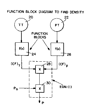
Figure 1 is a function block logic diagram which can
be utilized to determine the density of a fluid being
tested.-
Figure 2 is a graph illustrating pressure andtelnperature of the fluid being tested; the graph is divided
into subregions to improve the accuracy of the resulting
measurement of the fluid property being investigated.
lOFigure 3 is a graph of the temperature correction
factor ~CF)T versus temperature for the fluid being tested.
Figure 4 is a graph of the pressure correction factor
(CF)p versus pressure for the fluld being tested.
Figure 5 illustrates the logic blocks and the
15temperature correction factors for subregion 1 and 2
illustrated in Figure 2.
Figure 6 is a logic diagram for multiple temperature
and pressure subregions to determine the density of a
fluid.
20Figure 7 is a logic diagram of the subregion logic
block illustrated in Figure 6.
Figure ~ is a logic diagraln of the temperature
correction logic block illustrated in Figure 6.
Figure 9 is a logic diagram of the reference logic
25block illustrated in Figure 6.
Figure 10 is a graph of percent error versus
temperature illustrating the ilnproved mcasureinent accuracy
which is achieved by utilizing a dynalnic correction factor.
~0~4~
, . . .
--4--
--- OESCRIPTION OF THE P~l~FEl~l~EI) I~M~()L)IMEN'l'
Referring now to the drawings where the illustrations
are for the purpose of describing the preferred embodiment
of the present invention and are not intended to limit the
inYention described herein, Figure 1 is a logic diagram of
the functions required to determine the density of a
fluid. The foregoing density determination requires a
temperature transmitter 20 and a pressure transmitter 22
whose outputs are connected to the inputs to function blocks
24 and 26, respectively. The outputs of function blocks 24
and 26 represent the corrections factors (CF)T and (CF)p
for the temperature and pressure, respectively, of the fluid
being tested. The foregoing outputs are applied as inputs
to multiplier 28 whose output is connected to an input to a
multiplier 30. Another input to multiplier 30 is the
initial density ~ of the fluid being tested. The output of
function block 30 is given by the following equation:
~: ~O(cF)T (CF)p (1)
.
where,
~ = density
(CF)T;(CF)p = corrections factors for T and P
T = temperature
P = pressure
Also, the corrections factors are assumed as,
(CF)T = ~ (T,Po)/pO (2~
( F)p ~ (To,P)/~o (3)
~2~g~
J
where, _
(T,Po) = density values when T varies and
P = P
- o
(To,P) = density values when P varies and
T = T
o
The foregoing correction factors can be illustrated by
functional relationships (curves). It should be noted that
the values for correction factors (CF)T and (CF)p are unity
for P = PO and T = To (reference values) and in this case
density is ~ through Equation 1. The values for the
correction factors (CF)T and (CF)p are also obtainable
through fluid property tables. It should also be noted that
enthalpy and entropy values can also be determined in real-
time by the same approach.
The logic functions required to determine fluid
density ~ from temperature T and pressure P measurements is,
as previously discussed, illustrated in Figure 1 for a
single subregion (telnperature T an(l ~ressure P) of
operation. For multiple temperature and pressure
subregions, the method of implementation is best described
by an example. Consider a steam operating region having
boundaries between 350-450C and 4000~6000 kpa. Assume
further that this operating region can be divided into four
equal subregions specified as one throug'n four, as shown in
Figure 2. Fluid density ~ will be calculated in this
example since it has the tendency to produce the greatest
error.
- 2Q28~
~--Considering "Subregion 1" in Figure 2, the correction
factors set forth in Equations (2) and ( 3) ars illustrated
in Figures 3 and 4, respectively. The functional
relationships of the correctlon factors are produced by
function blocks 24 and 26 for temperature T and pressure P
falling within Subregion 1. It should be noted that the
reference values for Subregion 1 are To = 375 C and PO =
4500 kpa
The same approach can be taken for each of the
Subregions 2 through 4 in Figure 2. The temperature
correction factors (CF)T and (CF)T for Subregions 1 and 2,
respectively, are shown in Figure 5(b~ whereas the
t t
temperature logic representations fT and fT, for Subre(3ions
1 and 2, respectively, are shown in Figure 5(a).
Corresponding pressure logic representations fp and fp for
pressures 400C-5000 kpa and 5000-6000 kpa in Subreyions 1
and 2, respectively, can be developed.
Figure 6 illustrates the logic diagram for determining
the value of density ~ for multiple temperature and pressure
subregions. As such, this Figure includes a subregion logic
block 30, a temperature correction logic block 40, a
reference logic block 50, a pressure correction logic block
and a portion of the logic diagram shown in Figure 1.
The subregion logic block 30, illustrated in Figure 7,
contains four logic functions: two for temperature, as
shown in Figure 5(a~, and two for pressure. Only one of the
outputs of subregion logic block 30 is actuated at a time,
and the output that is actuated corresponds to the subregion
determined by the temperature and pressure of the fluid
being tested. The values of the other outputs of the
subregion logic block 30 are zero. The outputs of the
subregion logic block 30 are used as inputs to the
temperature correction logic block 40, illustrated in Figure
8, which produces temperature correction factors.
2 ~
.
The_ temperature correction factor functions ~7ithin logic
block 40 are arranged so as to receive the output signals
produced by the subregion logic block 30 and to produce the
proper value of the temperature correction factor (CF)T
depending upon the subregion being utilized. In order to
accomplish the foregoing, the temperature correction factor
functions within logic block 40 are biased by the output of
the temperature transmitter 20. It should be noted that the
pressure correction factor (CF) is determined in a similar
manner in pressure correction logic block 60.
In a similar manner, the reference logic block 50,
illu3trated in Figure 9, is utilized to produce a reference
density ~O based upon the output of the subregion logic
block 30 and the initial value of the fluid density ~O for
the subregion being utilized. The foregoing three output
signals, (CF)T, (CF~p and initial fluid density, are then ~ -
combined as shown in Figure 6 and in accordance with
Equation 1 to produce a measurement of the density f of
the fluid under test.
The accuracy of the resulting measurement of fluid
density can be improved by implementing a modified form of
Equation (1) which can be referred to as "dynamic
correction", as shown below: :
pc ~ [(CF)T (CF)p]n (4)
where, n is function of temperature T and pressure P
according to the following equation:
n = f(P,T) (S)
~;2~
.
.. . .
For- a particular fluid, values oE n are determined for a
different values of pressure P and temperature T and the
minimum error between table values and calculated values are
noted. In determining the foregolng function, a curve
fitting procedure is used. Through experimentation for
steam properties, it has been found that the values for n to
provide the desired accuracy can be achieved when n is a
function of only T as shown below:
n fT~ ) (6)
The improved accuracy ~hrough "dynalnic correction" along
with a representation of the relationship n = fT(T) is
illustrated by the curve in Figure 10.
It should be noted that measurement accuracy is
greatly improved by using the form of Equation (4) instead
of the form of Equation (1~ in Figure 1. The details of
providing the value of n for Equation (4) and implementing
same is similar to what has been previously presented.
The foregoing method of measuring fluid properties has
a number of advantages. For example, the accuracy of the
resulting measurements is determined by the size of the
measurement region and thus, accuracy can be controlled.
Considering steam as the fluid under test, a maximum error
of within .01% is easily obtained for a measurement
temperature range of 50C and a rneasurement pressure range
of 1 mpa. The total range of telnperature and pressure does
not affect the accuracy of the results inasmuch as the same
temperature and pressure measurement ranges can be
maintained by developing multiple pressure and temperature
subregion~. In addition, the foregoing "dynamic correction"
factor is utilized to modify the values of the correction
factors in order to further reduce measurement erxor. It
.. .. . - ., .... ~ , . ..
~2~
_9_
has ~-been found that by using this correction factor, the
maximum measurement error can be reduced by up to 50%.
Thus, an accuracy of within .005% can be obtained through
the use of the foregoing dynamic correction factor. It
should be noted that such improved accuracy does not
significantly increase costs.
In summary, the primary advantage of the foregoing
method is an increased accuracy in the resulting fluid
property measurements which are in real-time. The resulting
measurement accuracy is a significant improvement over the
prior art approaches and results in increased product
quality and energy efficiency.
Certain modifications and improvements will occur to
those skilled in the art upon reading the foregoing. It
should be understood that all such modifications and
improvements have been deleted herein for the sake of
conciseness and readability, but are properly with the scope
of the following claims.