Note : Les descriptions sont présentées dans la langue officielle dans laquelle elles ont été soumises.
1 5-NM-3501
G . Gl over
E. Schneider~
METHOD FC)R RAP ID MAGNET SHIMMING
This invention relates to nuclear magnetic resona~ce
(NMR) imaging methods and apparatus and more particularly to
a method of shimming ~he magnets used wi~h such apparatus.
In an NMR imaging sequence, a uniform polarlzing
magnetic field Bo is applied to an imaged object along the z
axis of a spatial Carte~ian reference frame. The effect of
the magnetic field Bo is to align some of the object's
nuclear spins along the z axis. In such a field the nuclei
resonate at their Larmor frequencies accordlng to the
following equation:
~ y Bo (1)
where ~ is the Larmor frequency, and y is the
gyromagnetlc ratio which is conqtant and a property of the
particular nucleua. The proton~ of water, because of their
relative abundance in biological ti55ue are of primary
interest in NMR imaging. The value of the gyromagnetic ratio
y for the protons in water is about 9.26 k~z/Gauss.
Therefore in a 1.5 Teqla polarizing magnetic field B~, the
resonance or Larmor frequency o'f proton~ is approximately
63.9 MHz.
In a two-dlmen~ional lmaging sequenc~, a spatial z axis
magnetic field gradient (Gz) is applied at the time of a
narrow bandwidth ~Y pulBe guch tha~only the nuclei in a
:
,, , . ~ . , , . , "
.
' ' , . . . . . .
- , . :, . . :
, : , , , ~. ;. ,
, ' , : , , .
.. . .
15N~35~
slice through the ob~ect in a planar slab orthogonal ~o the
z-axis are excited into re~onance. Spa~ial informaLion is
encoded in ~he resonance of these excited nuclei by applying
a phase encoding gradien~ (Gy) along the y axis and then
acquiring a NMR signal in the presence of a magnetic field
gradient ~Gx) in the x direction.
In a typical two dimensional imaging sequence, the
magnitude of the ph2se encoding gradient pulse Gy is
incremented between the acquisi~ion3 of each N~R signal to
produce a view set of NMR data from whlch a slice image may
be reconstructed. An NMR pulse gequence is d~cribed in the
article entitled: "Spin Warp NMR Imaging and Applications to
Human Whole Body Imaglng" by W. A. Edelstein et al., ~hYsi~5
~ L-=-I LYI~3~1~9~ Vol. 25 pp. 751-756 ~1980).
The polarizi~g magnetic field 30 may be produced by a
number of types of magnets including: permanent magnets,
resis~ive electromagnet~ and superconducting magnets. The
latter, superconducting magnet~, are particularly desirable
because ~trong magnetlc fields may be main~ained without
expending large amount~ of energy. For the purpose of the
~ollowing dlscus3ion, it will b,e a3sumed that the magnetic
field Bo i~ mainta~ned within a cyl~ndF~cal magnet bore tube
whose axis i-~ allgned with the z-axl~ referred to above.
The accuracy~of the image ~ormed by NMR imaging
25 techniqueg i3 highIy dape~dant o~ the uniformlty of this
polariz$ng magnetic field 80. Mo~t ~tandard NMR imaging
. ` . , ~ , ` ` . .
15N~03~01
technique~ require a field homogeneity better than ~4 ppm
(~250 ~) at 1.5 Tesla o~er the volume of interest, located
within the magnet bore.
The homogeneity of the polarizing magnetic field Bo may
be improved by shim coils, as are known in the art. Such
coils may be axis~symmetric with the z or bore axis, or
transverse ~o the z or bore axiQ. The axis-symmetric coils
are generally wound around a coil form coaxial with the
magnet bore tube while the transverse coils are generally
disposed in a so-called saddle shape on the surface of a coil
form. Each such shim coil may be designed to produce a
magnetic field corresponding to one spherical harmonic
(nassociated Legendre polynomial~) of the magnetic field 90
centered at the isocenter of the magnet. In combination, the
~him coils of different order spherical harmonics may correct
a variety of inhomogenei~ies. Among the lowe~t order shim
coils are those which produce a linear gradien~ along one
axis of the spatial refarence frame.
Correctlon of the inhomogeneity of the polarizing field
~0 Bo involveq ad~u-~tment of the individual shlm coil currents
~o that the combined field~ of ~he ~him coil~ just balanoe
any variatlon in the polarizing field ~o to eliminate the
inhomogenelty. T~is procedure i~ often referred to a3
shlmming.
: . . .
- ., : ~ . .
,
` . ' . , ' , ' . ' , . . . . .
~' ' ' '' ' ~ :
. , . ' ,
.. ' . ' '
,
,"
15N~03501
Several methods of measuring the inhomogeneities of the
polarizing field Bo, and hence deducing ~he necessary shim
currents for each shim coil, have been used previously. In
one such method, me~surements of Bo are made by means of a
magneeometer probe which is sequentially positioned at each
measurement point. The inhomogeneitieq of B~ are determin~d
from a number of such mea~urementY. Repositioning the
magnetometer probe between readings, however, make this a
time consuming method. There~ore, thls me~hod is most often
employed in the initial ~tage-q of magnet ~etup when only a
coarse reduction in field inhomogenei~y is nece3sary and
accordingly only a few sampled points need be taken.
Another method of mea~uring the inhomogeneitie~ of the
polarizing field ~o, is described in U.S. Patent 4,740,753,
entitled: "Magnet Shimming U3ing Inormation Derived From
Chemical Shift Im2gingn, issued ~pril 26, 1988 and assigned
to the same a~signee as the pr~sent application. In this
method (nthe CSI method"), a phantom containing a uniform
material (water) i~ used to make magnetic field mea urements
at specific locat~on~ ("voxel3 n ) within the phantom. A
frequency qpectrum ia obtained at each voxel and the position
of the resonance line of water is determined. The
displacement of the ~esonance li~e p~ovide~ an indication o~
the inhomogeneity at ~hat voxel. TheQe 1nhomogeneity
!
" '
" ~ ~
', . . : ' . ' . :: :: '',. ;, : '
'', ,' , . :, ::;' '' . ' ' .
s~; ;
15NM~3501
measurements, for a limited number o~ points, are expanded
mathematically to providP a map of the inhomogeneities over a
volume within magnet bore.
The CSI method is more accurate and much faster than
that of repositioning of a magnetometer probe within the bore
of the magnet. Nevertheles~, the CSI method ha~ a number of
shortcomings: Firqt, the signal-to-noise ra~io of the
acquired spectra at each voxel must be high to provide
accurate determination of the spectral peak. This in turn
require~ that the size of the voxels in which the
inhomogeneity is determlned be relatively large. The large
size of the voxels reduce~ the ~patial reqolution of the
inhomogenei~y determination and adver~ely affect~ the
calculation o~ the higher order shimming field~.
Second, the acqui~ition ~ime for each spec~rum ls
relatively long. AY is generally under tood in the art, the
frequency reqolutlon of the ~pectra i~ inversely proportional
to the length of t~me over which the NMR 3ignal i~ sampled.
A ~ufflc~ently well resolved spectrum ~or use in the CSI
method require~ an NMR acquisition tlm~ on the order of one
hal~ ~econd for each vox~l. Thi~ may be co~trasted with the
approximately d m~ readou~ per 256 voxel~ required in an
ordinary NMR imaging scan. A a result, the acqui~ition of
data for the above CSI m~hod requlres approximateLy S
minute~ per 16 by 16 voxel image, a rela~ively long tlme.
.
- . .
.
:
-. ~ ' ~, ' . ~ ' ' .
s?
15NM03501
Third, the processing of the sp~ctra to determine the
frequency locatlon of each spec~rum's peak al.so requires a
substantial amount of time.
The present invention relates to a method of measuring
the inhomogeneitieQ of a polari~ing magnetic field ~o
directly from two conventional NMR image-~ having different
phase evolution times. The inhomogenei~y data so derived may
be expanded against polynomials approximating the fields
produced by the shim coils. The coefficients of this
expansion may be used to determine the setting of the
currents in the shim coilq necessary to correct the
inhomogeneity.
Speciically, a ~irst and econd N~R view set is
acquired with a fir~t and seco~d, different evolution time
and tE2. A gradient echo or spin echo pulqe sequence may be
used. A correspo~ding fir3t and second complex multipixel
image i~ recon~tructed ~rom each NMR view set, a~d these two
image8 are divide~, one ~y the other on a pixel by plxel
ba~i~, to produce a complex mul~ipixel ratio image. The
argument of this complex multipixel ratlo image provides an
inhomogeneity map of the polarizing magnetic field, from ~ ~
which the compen~a~ing energization of the shim coil~ may be ~: -
determined.
:- - ' ' ,, - ' ' ' .
:
15N~3~01
The method of adjusting the shim coils may include
fitting the inhomogeneity map o~er a volume of interest ~o a
set of polynomials which approximate the fields produced by
the shim coils. The value o~ the coerficients of these
polynomials after the expansion will approximate the required
shim coil currents. Also, a calibration matrix describing
the deviation of the fields produced by each shim coil from
the asscciated polynomial may be determined and used in
conjunction with the coef~icients of the polynomials to
adjust the energization of the shim coils.
It i3 one object of the invention, therefore, to
decrea.~e the time needed to shim a NMR magnet from that
required by the previously descri~ed CSI method. The use of
two st~ndard NMR view image.~ rather than the chemical shift
image spectra used in the CSI method reduce the data
acquisition time substantlally with vastly increased
resolution. The sub~equent processing o~ the acquired image
data to determine the inhomogeneiky is also fa-~ter than the
peak finding p~ocedure of the CSI method.
It is another ob~ec~ of the invention to provide an
inhomogenelty mea3urement with better spatial resolution
than the CSI method. The method of the present invention is
less sen~ltive to the slgnal-to-noise ratio of the ~MR view
lmage.q and hence the ~nhomogene$ty of smaller voxel~ may be
mea~ured.
.
, ~' "
~J 1 ~
8 15NM03501
Other objects and advantage5 besides those discussed
above shall be apparent to those experienced in the art from
the description of a preferred embodiment of the invention
which follows. In the description, reference is made to the
accompanying drawings, which form a par~ hereof, and which
illustrate one example of the invention. Such example,
however, is not exhaustive of the various alterna~i~e forms
of the invention, and therefore reference is made to the
claims which follow ~he description for determining the
scope of the invention.
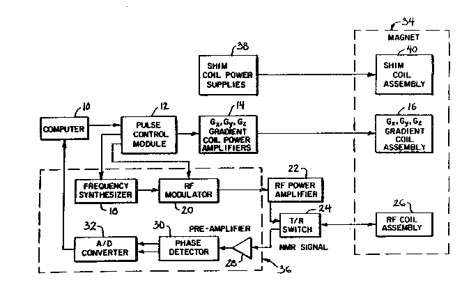
Figure 1 i~ a schematic block diagram of an NMR sys~em
suitable for the practice of thl4 invention;
Figure 2 is a graphic repr~sentation of a gradient echo
15 NMR pulse sequence; ~ :
Figure 3(a) i3 a three dimen~ional graph of measur~d
inhomogeneity Q' over an area o~ an x-y plane;
Figure 3(b) is graph of measured inhomogeneity Q' versus
x taken along a line of constant y through the three
dimen~lonal graph shown in F1gure 3(a);~
F~gure 3~c) i~ a graph of the partlal derivative of the
function graphed in Figure 3(b), ~howing the determlnation of
the polnta of dlscont~nu~ty by a ~hreshold1ng proce~s~
:
, ,
. .
- : ~ , . . ~ . :
. . : . , : -
- :
: - ~: '. , :: -
: : : :
15NM~3501
Figure 3(d) is a graph o~ the weighting function T~x)
used to reduce the discontinuities of the partial derivative
of Figure 3~c~ during curve fitting of shim fields.
~
~igure 1 is a block diagram of an NMR imaging system of
a type suitable for the practice of the invention. It should
be recognized, however, that the claimed invention may be
practiced on any suitable apparatu~.
A computer 10 controls a pulse control module 12 which
in turn controls gradient coil power amplifiers 14. The
pulse control module 12 and the gradient amplifier~ 14
together produce the proper gradient waveformq Gx, Gy~ and Gz,
as will be de~cribed ~elow, for a gradient echo pulse
sequence. me gradient waveforms are connected to gradient
coils 16 which are po~itioned around the bore of the magnet
34 so that grad1ents Gx, Gyr and Gz are impressed along their
respective axeQ on the polarizin~ magnet1c field Bo from
magnet 3~.
Th~ pul-Qe control module 12 also controls a radio
fLequency synthesi~er 18 which i~ part of a~ RF transceiver
system, portions of which are enclo~ed`by dashed line block
36. The pulse co~trol module 12 alqo controls a RE modulator
20 which modulateq the output of the ra~io requency
synthe izer 18. The resultant RE gignal3, amplified by power
amplifier 22 and applied to RF coll 26 through
:
15NM~3501
~ransmit/receive switch 24, are u~ed to excite the nuclear
spins of the imaged object (not shown).
The N~ signals from the excited nuclel of the imaged
object are plcked up by the RF coil 26 and presented to
preamplifier 28 through transmit/receive switch 24, tO be
amplified and then processed by a quadrature phase detector
30. The detected signals are digitized by an high speed A/D
converter 32 and passed to computer la for processin~ to
produce NMR images of the object.
A series of shim coil power supplies 38 provide current
to shim coils 40. Each shlm coil may generate a magnetic
fisld which can be de cribed in term~ of spherical harmonic
polynomials. The first order shim field can be produced by
either the gradient coil-~ 16 or the shlm coil~ 40, with
lS higher order shim fields produced by the sh~m coils 40 only.
The following dlscussion conslders a gradient echo pulse
sequence produced on the above de cribed apparatu and
suit ble for u-Re w$th the pregen~ invention. It should be
under~tood, however, that the lnvention may be uQed with
other pulse sequences as wlll be apparen~ from:the following
discussion to one of ordlnary skill in the art.
Referring to FLgure 2, a gradtent echo pU19~ sequence
begins with the transmtS lon of a narrow bandwidth ~adio
frequency (RF) pu1se S0 ln the pre~ence of s11ce selection G~
:'
~:
-:
11 15NM03501
pulse 52. The energy and the phase o~ this initial RF pulse
may be controlled such that at its termination the magnetic
moments of the individual Quclei are aligned in the x-y plane
of a rotating reference ~rame of the nuclear spin system.
S pulse of such energy and duration is termed a 90~ RF pulse.
The rotating frame differ~ from th~ previously described
spatial reference frame in that the rotating frame rotates
about the spatial z-axi~ at a ~requency ~o equal to the
Larmor frequency of the dominan~ proton species without any
additional shim fields.
The result of the combined RF signal and gradient pulse
52 is that the nuclear spins of a narrow slice in the ~hree
dimensional imaged object along spatial z-plane are excited.
Only those spins with a Larmor frequency, und~r th~ combined
field Gz and Bo~ within the frequency bandwidth of the RF
pulse will be excited. Hence the position of the slice may
be controlled by the gradient Gz intensity and the RF
frequency.
A negative Gz rewinder gradient pulse 54, serves to
rephase the nuclear spins in the x-y plane of the rotating
fra~e. Rewinder pul~e 54 therefore iq approximately egual to
half the area of that portion of qlice selec~ gradient 52
which occurY during the RF puIse 50.
After or during the application of the Gz reuinder pulse
54, the Gx prewlnder pul~e 56 i~ applied. Tbe prewinder
pulse 56 begins ~o dephase the prec~s~ing nuclei: those
,: . : -
.
12 15NM03501
nuclei at higher spatial locations wi~hin the ~lice ad~ance
in phase faster as a result of the Gx-induced higher Larmor
frequency than those nuclei at lower spatial locations. .
Subsequently, a positive ~ readout pulse 58, cen~ered a~
time tE after the center of ~F pulse 50 causes the dephased
spins to rephase into a gradient echo or NMR signal 60 at or
near the cen~er of the read-out pulse 5~. The gradient echo
60 is the NMR signal for one row or column in the ima~e.
In a two dimensional imaging sequence, a gradient pulse
Gy 6~ is applied to phase encode the spin~ along the y axis
durinq the prewinder gradient 56. The sequence is then
repeated with different Gy gradien~s, a~ is unders~ood in the
art, to acquire an NMR view set ~rom which a tomographic
image of the lmaged ob~ect may be reconatructed according to
conventional recon~truc~ion techniques.
The NMR slgnal 60 is the sum o~ the~component signals
~rom many precessing nuclei throughout the excited slice.
Ideally, the phase of each component 4ignal will be
determined by the strength of the Gz, Gx and ~y gradients at
the location of the individual nuclel during the read out
pulse 58, and hence by the spatial z-axis, x-axi~ and y-axis
location~ of the nuclei. In practice, however; numerous
other factors affect the phase of:the NMR aignal 60.
For the purpo~e3 of ~implifying the followin~ di~cussion
of N~R signal phag~ w~l be aggum d t~at th~ abJect beinq
, : . , ~ .: ~ :. .
.
-. . ... . .
. .
13 15NM03501
imaged has no variation in the y direction. The NMR signal
60 may be then represented as follows:
S(t) = ¦ p(x)ei~xxt-eiyBo(~+t).ei~x~(tE+t).ei~ dx (2)
where p(x) is the spin density, i.e. the number of
nuclei at a given voxel in the x direction; y is the
gyromagnetic constant of the nuclei of the material being
imaged; Bo is the strenyth of the polarlzing magnetic field;
G~ is the slope of the x axis gradient and tE is the phaqe
evolution time described above.
The first complex term of thiq integral, e
represents the effect of the readout gradient 58 o~ the NMR
signal S(t). The gradient pr@winder 56, causes this effect
to be referenced not from the start o the gradient pulse 58
but from to the cen~er of the gradient pulse 56 aq qhown in
lS Figure 2.
The second complex ~erm of this equa~ion, ei~tE+t),
repreqent~ the effect of the polarizin~ field ~o on the NMR
signal S~t). Bo i continuou ly presen~ and hence, in the
gradient echo pulse sequence, the eSfect o~ Bo on S~t) i~
measured from the lnstan~ o~ occurrence of the ~F pulse 50.
The time elap~ed .~lnce the RF pulse S0, in the gradient echo
pulse sequenCe is ~E+t a~ shown ~n Figure 2.
The third complex ter:m o2 thl~ e~uation, elQ(~)(tE~t)~
arise~ from 1nbomogeneitie~ in the magne~lc ~ield ~o. These
~.
~. ~
.
: ,
15~03501
14
inhomogeneitles are generally spatlally variable and may be
derived from the second complex term of equation (2).
Specifically ei~tE+t) becomes e~Y~B~3(X)~(tE~t~ where ~B~x)
is the inhomogeneity of 80 and generally a function of x.
This inhomogeneity function may be factored into a separate
complex term ei~(X~(tE~t) where Q(X~=Y~B and Q is termed the
actual inhomogeneity. The phase error of such
inhomogeneities in 80 increases for increa ~ng phase evolution
time and hence this term is a function of t~+t, for the same
reasons as those described above for the second complPx term
of equation (2).
The fourth compLex term of thi~ equation, ei~, collects
pha~e lags or leads requlting from ~Ae signal procsssing of
tAe NMR signal chain. For example, the RF coil structure 26,
shown in Fiqure 1, may introduce cer~ain phase diqtortions as
may the RF power amplifier 22 and the preamplifier 28. These
phase term.q may also vary with x and are repre~ented by the
term ei~.
This equation (23 may be ~implified by recognizing ~hat
the NMR signal is typically hetrodyned or shifted in
frequency to remove the base frequency of water polarlzed by
the magnetlc field Bo. Thi frequency shift tran3formation
i~ accomplished by multiplying S(t) by e~i~dtE+t) producing
t~e ~ignal S'~tl:
S'~tl ~ ¦ p~x)e1~xX~-elQ~x)(tE+~j e~0 dx (3)
,
15NM03S01
The following substitution is now made to simplify the
reverse Fourier transformation necessary to produce an image
from S'tt):
x=x ' -~2 ( x ) /~x
yielding
S'(t) 3 ei~-Jp~ Q(x)/~yGx)el~;xx~t.ein~x~)(tE) ~X~ (S)
The reconstruc~ion, a3 mentioned, is performed by
performing the reverse Fourier transform upon S'(t) to derive
a complex, multipixel image P~x)':
P(x) ' ~IS' (t~e~i~xXtdt
~ei~-(p(Xl-Q(X)/rG~).eLQ~x~)(t~ (6)
The pixels of the image P(x)' are displ~ced from their
true positions x by the term u-~ed in the cubstitution given
in equation (4), however thl~ displacement may be ignored if
lS the di~placement is on the order of one pixel. A
displacement of le~s than one pixel will result if the
inhomogeneity ~B of the magnetic field 30 i~ ~mall relative
to the gradlent strength Gx~ S~eclfically if Q(x)/~x < one ~
pixel or by ~he previous definition of Q5x) in terms of ~B, ~` .
2C ~3(x)~Gx< one pixel. For a 1.5 Te~la magr~et wi~h a Bo ~ield
of approxima~ly S00,000 time the lncrement in gradient
field pèr pixal, th~ pixel displaoemen~ wlll be on the order
.. " ~
~s',;~,'~,l~,,
16 15NM03501
of one pixel if the magnet ha~ an initlal homogeneity of 2
ppm. The term ~/yGx is then approximately 1.7 and may be
ignored in area~ of the imaged object where there there is
little change in ~he signal from pixel to pixel as will
generally be the case with a phantom. As will be described
further below, the expansion process will tend to further
decrease error resulting from occasional deviations from
these assumptions.
Assuming the pixel displacements may be ignored,
equation ~6) becomes:
P~x)l=p~x)ei~(x)(~.ei~ (7)
The inhomogeneity da~a Q may be extracted by per~orming
two experiments and producing two signals Pl~x) and P2(x) with
two different evolution time3 tE1 and ~E~. The difference
between t~l and t~2 will be termed ~ and lts selection is
arbitrary sub~ect to the following con5~raint~: larger values
of ~ increa~e the re olution of the measurem~nt of
inhomogeneity but cause the inhomogeneity data n to "wrap
around~ with large magnetic field inhomogeneitieS.
Conversely, smaller value~ of ~ decrease the resolution of the
mea~uxement of inhomogenei~y but permit the measurement of
larger magnet inhomogeneitie~ without "wrap aroundN. Wrap
arounds result~ from the per~odicity of ~he trigonometric
functionq used to calculate ~he lnhomogeneity data Q a will
be de~cribed in more detail below.
:
~ r ~ ~
17 15N~03501
For these two experiments with different e~olution times
t~l and t~2:
Pl(x)=p(x)eiQ~x)(tEl).ei~. (8)
and
S P2 (X) ap (X~ ein~X)(tE2)
p ( x) eiQ ~X) (tEl~
= PleiQ~x)~ (9)
A third image P3 may be then produced by dividing imag~
P2 by Pl, on a pixel by pixel basis, such that
P3(x)~ P2 _ eiQ~x)~ (10)
~(x)3arg(P3(x)) (11) .
Thus P3 is an image whose argument~A~, (the angle of the
complex number ei~X~t) is prop~rtional to the inhomogeneity
Q(x). The inhomogeneity Q(x~ may be calcula~ed at~any point
x by dividing ~x), the argument of P3~x) at the pixel
a soctated wlth x, by ~.
A~ ha~ now been described, the argument ~(x) o~ the
complex lmage ~3 divided by ~ yieid~ a map of~the~
inhomogeneity Q(x) over the image~P3'~ sur~ace. The complex
array P3 is represented digitally ~ithln the~NMR system by
means of two quadrature array9 indlcating the magnltud~ of
ine and coslne~terms o~ P3 respectlvely. The:argument or
lB 15NM03501
phase angle of P3 may be extrac~ed by application of the
arctangent func~ion to the ratio of these quadrature arrays.
The arctangent function ha~ a range of -~ to +~ and therefore
the argument of ~(x) will be limited to values within this
range. The measured inhomogPneity Q' is equal to the
argument ~ divided by ~ and therefore the measured
inhomogeneity value Q' will be restric~ed to the range -~/~
to ~ . For values of the actual inhomogeneity Q outside of
thiq range, Q' will "wrap around'~.
Referring to Figure 3(a) an example map of measured
inhomogeneity Q'(x,y) 80 over a ~wo dimensional image P3(x,y)
is shown with Q'(x,y) plotted in the vertical dimension. The
actual inhomogeneity Q~x,y) increa~es mono~onically over the
surface P3, however, as explained, the measured inhomogeneity
lS Q'(x,y) is bounded between the arctangent lmposed limits of
~ to +~/~. Accordingly, disconttnuitie~ 81 occur at the
points where the arctangent function is discontinuous at ~
and -~. The actual inhomogeneity Q(x,y) may be determined by
by "unwrapping" the discontinuitie~, a complex topological
problem that requires tallying the di~continuitie~ aq one
moveQ ovex the surface of the P3(x,y) argument array 80 and
addlng or ~ubtracting 2~ to the measured inhomogeneity Q' as
each diqcontlnuity 81 i~ pa~ed.
This difficult talIying procedure may be avoided,
provided that the imaqe object ha~ only one proton species,
as would be the case with a phantom u~ed for ghlmming, if ~ is
;: :,, ,
. , , -
;
.. ~ . :: :
.
~`' t" . ~. /'.
19 15NM03501
chosen to be small enough to eliminate ~rap arounds.
Specifically, T ~1 , where ~v is the frequency spread of the
resonating protons across the measured volume caused by the
magnet inhomoge~eity. Once the initial inhomogeneity is
S corrected with this small value of ~, the process may be
repeated with larger ~ to improve the resolution of the
inhomogeneity measurement for subsequent iterations.
Alternatively, the wrap arounds may be detected and
corrected by taking the spatial partial derlvative-q of the
measured inhomog~neity map 80.
Referring to Flgure 3(b), the value~ 82 of the measured
inhomogeneity map Q'(x,y) 80, along a line parallel to the x
axis, are shown. Curve 82 rise~ with increasing Q',
associated with increasing ~alues x, until the ~' reacheq
+~/~ at which point it ~ump~ to ~ aa a result of the
previou~ly diqcussed di~continuitieq at ~ and -~.
A first partial derivative, &a'/~x, along line 82 is
shown in Figure 3(c). The partial derivative exhibit~
"-~pikeq~ 81' at the point~ of discontinuity ~1 in Fiqure
3~b). These polntQ o discontinuity may be readily detected
by comparing curve 84 to a thre-qhold value ~5 and creating a
weiqhting function T(x), a~ shown in Figure 3(d), whose value
i~ zero when the magnitude of curve 84 i~ gr0ater thon the
,,
, . : ,
; . . . . .
." ?
15NM03501
threshold value 85 and one otherwise. The threshold is
preferably set to ~/8~ although other valueg may be used. The
phase weighting function, T~x) is then used to fit the
derivative inhomogeneity data to spatial deri~atives of the
spherical harmonic polynomials aa will be described below.
In a further embodiment, an amplitude weigh~ing function
W(x,y) is also constructed such that the amplitude weighting
function W~x,y) equals zero when the magnitude of image value
P3 is less than a second threshold v~lue and one otherwise.
The second threshold is set to 15% of the maximum signal
magnitude within the area of the image under con~ideration,
although other value~ could be selected depending on the
signal to nolse ratio of the image. The amplltude weighting
function is u~ed to diminish the importance during expansion
of the inhomogeneity map $n areas where there is little
signal strength, as indicated by the magnitude o~ P3, and
hence serves to eliminate incoherent, irrelevant phase wrap
arounds ariQing from re~ion~ w$th no amplitude. As will be
appa~en~ to one of ordinary kill in the art, the weigh~ing
function W(x3 may be implemented in numerou~ other ways.
For example, W(x) may be a continuouq ~unction of the
magnitude of the lmage or the power o~ the image IP)2.
The a~Qociated Legendre polynomlals may be fit to the
inhomogeneity data by a we~ghted lea~t qquare3 method uslng
, .... .
~ ~ -
.'., ~ .
f,~ ' ~ " ', ';
,: ,, .,' : ',: ; .
~ . . ''.~ ' ' . ~
21 15NM03501
weighting fu~ctions T and W as described abov~ and as ls
understood in the art. If ~ i~ chosen such that no wrap
arounds occur, then the inhomogeneity data is fit to the
appropriate associated Legendre polynomials directly. If ~ is
chosen such that wrap arounds do occ-~r, the wrap arounds are
removed as deqcribed abo~e and ~he resultant differentiated
inhomogeneity data is fit to the appropriate differentiated
associated Legendre polynomials.
A straight forward least squares fittin~ of the data in
this manner carrieq the implicit assumption that the
inhomogeneitie~ are centered at the isocenter of the magnet.
Thls will not always be the case however, and if the
inhomogeneities are off center, the coefficient~ so
determined will lnclude errors if the full complement of
appropriate Legendre polynomials are noe used in the field
correction. Thiq distortion of the fitting may be corrected,
if the off~et is known, by spatially qhifting the associated
Legendre polynomial~ by the amount that the inhomogeneitie~
are off center. Specifically, a Taylor expansion of each
polynomial i~ performed by sub~tituting the variableq x-xo,
y-yo, and z-zo for x, y, z, where xo, yo, and zo are the
distance~ by which the center of the inhomo~eneitie~ are
offset from the i ocenter. Thi~ procedure effectlvely shift~
ehe polynomial~ ~o that they are centered on th~
inhomogeneity prior to th~ fittln~ proce~ being per~ormed.
. : : . ` ' - ~' , . ':
h~
22 15N~03501
It has been determined that the inhomogenelties tend to
be centered on the cen~er of maQs of the imaged ob~ect. This
follows from the effect that the pregence of the imaged
ob~ect has on the magnetic field lines. Accordingly the
center of mass o the imaged objec~ is first determined from
the amplitude of the image So~x,y). Specifically, for the x-
axis:
¦ISo~x,y)lxdxdy
xo ~ _ _ (12
¦ISo ~x,y)ldxdy
The-valueq of y~ and zo are determined in a similar
manner.
The inhomogeneity data acquired in ~he above manner may
be used to determine the proper set~lng~ of the shim coils.
The technique of determ~ning the setting of the shim coils
from inhomoganeity data is degcribed in detall in the
previously cited U.S. Patent 4,740,753 a~ column 6 lines 62
8~ ~e~. and 1~ hereby incorporated by reference. This
proces~ i3 ~ummari~ed as follow~:
T~e in~omogeneity data or 'derivatLve data corrected by
the weighting~ function provide.~ a set of inhomogenei~y
measurement~ within a plane determined by the gradients of
the imzging sequence o~ Figu~e 2. Additlonal data i8
obtained for plane~ rotated about thc z-axla by 45, 90, and
:: :
-
. : .
- . .
23 15N~03501
135 to provide inhomogenelty measurements within the volume
of a cylinder radial symmetric about the z-axis. The
rotation of the imaging plane is obtained by simultaneous
excitation of the gradients wlth various factors applied to
the amplitudes as known in the art.
This collection of inhomogeneity measurements may be
expanded throughout a volume o~ intere~t as a series of
spherical harmonics or the spatial der~va~ive~ thereof. A
variety of polynomials may be used, however, the polynomials
are pre~erably related to the fields produced by the shim
coils 4Q. In the imaging sy~tem of Figure 1, the shim coils
40 are designed to produce fields approximating those
described by orthonormal aasociated Legendre polynomials and
hence associated Legendre polynomlal~ (nspherical harmonic
polynomials") or their spatial derivative-~ (if the above
unwrapping procedure was used) are used for the calculation
of the currents to be applied to the shim coils. The above
proceqs involves fittin~ the inhomogeneity meaqurements to
the polynomial~ or their ~patial deriva~ives by a~iusting the
coef~icient3 of the polynomialq according to a least squares
minimization or other well known curve fi~tlng proceqs.
Once thi-q proce~s ig compl~ted, the coefficients of th~
polynomials may be used to set the curren~-~ in ~he shim coils
to correct the inhomogene~ty per a calibration matrix as will
2S be now described.
- : . . . : : .
,
- , , ~, . .
24 15NM03501
Ideally the fields of the shim coils ~0 a~e de igned to
be orthonormal, tha~ is, each will correct a different
component in the spherical harmonic polynomial. In this case
the currents in the shim coils 40 would be proportional to
the coefficients of the corresponding polynomials. However,
to the extent that there iR some interaction between the
fields produced by the shim coils 40, i.e, a given shim coil
40 produces magnetic field components in other harmonics than
its own, a calibration matrix must be determined. The
calibration matrix is produced by measuring, individually,
the effect of each shim coil 40 on ~he magne~ic field
homogeneity. The currents in the shim coils m~y be then
determlned by meanY of ~he calibration matrix and the
polynomial coef~icient3. Any remaining error may be
corrected by repeatin~ the entire proce~s for ~everal
iterations.
While this invention haQ been de~cribed with reference to
particular embodimentQ and examples, other modifications and
variationq, Quch as application to pro~ectlon reoonstruction
imaging technique~, will occur to those ~killed in the art in
view of the above teachings. For example, the technique may
be used with a phantom containing two chemical specieq or for
in-vivo shimming making use of the techniqueY ~aught in co-
pending U. S. paten~ application serlal number 07/441,850,
filed November 27,1989, en~itled: "M~thod For In-Vivo
Shimming" and assigned ~o th~ ~ame as~ignee a~ the pre~ent
,
~ :, . ' '
.,
15NM~3501
invention. Also, pulse sequences other than gradient echo
pulse sequences may be used, aq will be understood from this
discussion and a review of the techniques taught in the
previously cited application. Accordingly, the present
5 invention is no~ limlted to the p~eferred embodiment
described hereln, but is in~tead defined in ~he following
claims.
,- .
,
.