Note : Les descriptions sont présentées dans la langue officielle dans laquelle elles ont été soumises.
CA 02315814 2000-06-21
WO 99/34316 PCTNS98/27374
ENERGY MINIMIZATION FOR CLASSIFICATION, PATTERN
RECOGNITION, SENSOR FUSION, DATA COMPRESSION,
NETWORK RECONSTRUCTION AND SIGNAL PROCESSING
CROSS REFERENCE TO RELATED APPLICATIONS
This application claims priority of U.S. provisional application serial
number 60/071,592, filed December 29, 1997.
COPYRIGHT NOTICE
A portion of the disclosure of this patent document contains material which
is subject to copyright protection. The copyright owner has no objection to
the
facsimile reproduction by anyone of the patent document or the patent
disclosure,
as it appears in the U.S. Patent and Trademark Office patent file or records,
but
otherwise reserves all copyright rights whatsoever.
APPENDIX
An appendix of computer program source code is included and comprises
22 sheets.
The Appendix is hereby expressly incorporated herein by reference, and
contains material which is subject to copyright protection as set forth above.
BACKGROUND OF THE INVENTION
The present invention relates to recognition, analysis, and classification of
patterns in data from real world sources, events and processes. Patterns exist
throughout the real world. Patterns also exist in the data used to represent
or
convey or store information about real world objects or events or processes.
As
information systems process more real world data, there are mounting
requirements to build more sophisticated, capable and reliable pattern
recognition
systems.
Existing pattern recognition systems include statistical, syntactic and neural
systems. Each of these systems has certain strengths which lends it to
specific
applications. Each of these systems has problems which limit its
effectiveness.
CA 02315814 2000-06-21
WO 99/34316 PCT/US98/27374
2
Existing pattern recognition systems include statistical, syntactic and neural
systems. Each of these systems has certain strengths which lends it to
specific
applications. Each of these systems has problems which limit its
effectiveness.
Some real world patterns are purely statistical in nature. Statistical and
probabilistic pattern recognition works by expecting data to exhibit
statistical
patterns. Pattern recognition by this method alone is limited. Statistical
pattern
recognizers cannot see beyond the expected statistical pattern. Only the
expected
statistical pattern can be detected.
Syntactic pattern recognizers function by expecting data to exhibit
structure. While syntactic pattern recognizers are an improvement over
statistical
pattern recognizers, perception is still narrow and the system cannot perceive
beyond the expected structures. While some real world patterns are structural
in
nature, the extraction of structure is unreliable.
Pattern recognition systems that rely upon neural pattern recognizers are an
improvement over statistical and syntactic recognizers. Neural recognizers
operate by storing training patterns as synaptic weights. Later stimulation
retrieves these patterns and classifies the data. However, the fixed structure
of
neural pattern recognizers limits their scope of recognition. While a neural
system
can learn on its own, it can only find the patterns that its fixed structure
allows it to
see. The difficulties with this fixed structure are illustrated by the well-
known
problem that the number of hidden layers in a neural network strongly affects
its
ability to learn and generalize. Additionally, neural pattern recognition
results are
often not reproducible. Neural nets are also sensitive to training order,
often
require redundant data for training, can be slow learners and sometimes never
learn. Most importantly, as with statistical and syntactic pattern recognition
systems, neural pattern recognition systems are incapable of discovering truly
new
knowledge.
Accordingly, there is a need for an improved method and apparatus for
pattern recognition, analysis, and classification which is not encumbered by
preconceptions about data or models.
CA 02315814 2000-06-21
WO 99/34316 PCT/US98/Z7374
3
BRIEF SUNIfMARY OF THE INVENTION
By way of illustration only, an analyzer/classifier process for data
comprises using energy minimization with one or more input matrices. The data
to be analyzed/classified is processed by an energy minimization technique
such
S as individual differences multidimensional scaling (IDMDS) to produce at
least a
rate of change of stress/energy. Using the rate of change of stress/energy and
possibly other IDMDS output, the data are analyzed or classified through
patterns
recognized within the data. The foregoing discussion of one embodiment has
been
presented only by way of introduction. Nothing in this section should be taken
as
a limitation on the following claims, which define the scope of the invention.
BRIEF DESCRIPTION OF THE DRAWINGS
FIG. 1 is a diagram illustrating components of an analyzer according to the
first embodiment of the invention; and
FIG. 2 through FIG. 10 relate to examples illustrating use of an
embodiment of the invention for data classification, pattern recognition, and
signal
processing.
DETAILED DESCRIPTION THE PRESENTLY PREFERRED
EMBODIMENTS
The method and apparatus in accordance with the present invention provide
an analysis tool with many applications. This tool can be used for data
classification, pattern recognition, signal processing, sensor fusion, data
compression, network reconstruction, and many other purposes. The invention
relates to a general method for data analysis based on energy minimization and
least energy deformations. The invention uses energy minimization principles
to
analyze one to many data sets. As used herein, energy is a convenient
descriptor
for concepts which are handled similarly mathematically. Generally, the
physical
concept of energy is not intended by use of this term but the more general
mathematical concept. Within multiple data sets, individual data sets are
CA 02315814 2000-06-21
WO 99/34316 PCT/US98/27374
4
characterized by their deformation under least energy merging. This is a
contextual characterization which allows the invention to exhibit integrated
unsupervised learning and generalization. A number of methods for producing
energy minimization and least energy merging and extraction of deformation
information have been identified; these include, the finite element method
(FEM),
simulated annealing, and individual differences multidimensional scaling
(IDMDS). The presently preferred embodiment of the invention utilizes
individual
differences multidimensional scaling (IDMDS).
Multidimensional scaling (MDS) is a class of automated, numerical
techniques for converting proximity data into geometric data. IDMDS is a
generalization of MDS, which converts multiple sources of proximity data into
a
common geometric configuration space, called the common space, and an
associated vector space called the source space. Elements of the source space
encode deformations of the common space specific to each source of proximity
data. MDS and IDMDS were developed for psychometric research, but are now
standard tools in many statistical software packages. MDS and IDMDS are often
described as data visualization techniques. This description emphasizes only
one
aspect of these algorithms.
Broadly, the goal of MDS and IDMDS is to represent proximity data in a
low dimensional metric space. This has been expressed mathematically by others
(see, for example, de Leeuw, J. and Heiser, W., "Theory of multidimensional
scaling," in P. R. Krishnaiah and L. N. Kanal, eds., Handbook of Statistics,
Vol. 2.
North-Holland, New York, 1982) as follows. Let S be a nonempty finite set, p a
real valued function on S x S ,
p:SxS-~R.
p is a measure of proximity between objects in S. Then the goal of MDS is to
construct a mapping f from S into a metric space (X, d),
f :S->X,
CA 02315814 2000-06-21
WO 99/34316 PCT/US98/27374
such that p(i, j) = pij ~ d( f (i), f ( j)), that is, such that the proximity
of object i to
object j in S is approximated by the distance in X between f (i) and f ( j) .
X is
usually assumed to be n dimensional Euclidean spaceR", with n sufficiently
5 small.
IDMDS generalizes MDS by allowing multiple sources. For k =1, . . ., m let Sk
be
a finite set with proximity measure pk , then IDMDS constructs maps
fk'Sk-~X
such that pk (i, j ) = pjk ~' d ( fk (L ), fk ( j )) , for k =1, . . . , m .
Intuitively, IDMDS is a method for representing many points of view. The
different proximities pk can be viewed as giving the proximity perceptions of
different judges. IDMDS accommodates these different points of view by finding
1 S different maps fk for each judge. These individual maps, or their image
configurations, are deformations of a common configuration space whose
interpoint distances represent the common or merged point of view.
MDS and IDMDS can equivalently be described in terms of transformation
functions. Let P = ( p~ ) be the matrix defined by the proximity p on S x S .
Then
MDS defines a transformation function
f'Pij Hd;j(X)~
where d ~ (X ) = d ( f (i ), f ( j )) , with f the mapping from S --~ X
induced by the
transformation function f. Here, by abuse of notation, X = f (S) , also
denotes the
image of S under f . The transformation function f should be optimal in the
sense
that the distances f ( pj ) give the best approximation to the proximities pj
. This
optimization criterion is described in more detail below. IDMDS is similarly
re-
CA 02315814 2000-06-21
WO 99/34316 PCT/US98/27374
6
expressed; the single transformation f is replaced by m transformations fk .
Note,
these fk need not be distinct. In the following, the image of Sk under f k
will be
written Xk .
MDS and IDMDS can be further broken down into so-called metric and
nonmetric versions. In metric MDS or IDMDS, the transformations f ( fk ) are
parametric functions of the proximities p~ ( p~k ) . Nonmetric MDS or IDMDS
generalizes the metric approach by allowing arbitrary admissible
transformations f
( fk ), where admissible means the association between proximities and
transformed proximities (also called disparities in this context) is weakly
monotone:
P; ~ Pkr implies f ( pij ) <_ f (Pkr ) ~
Beyond the metric-nonmetric distinction, algorithms for MDS and IDMDS
are distinguished by their optimization criteria and numerical optimization
routines. One particularly elegant and publicly available IDMDS algorithm is
PROXSCAL See Commandeur, J. and Heiser, W., "Mathematical derivations in
the proximity scaling (PROXSCAL) of symmetric data matrices," Tech. report no.
RR-93-03, Department of Data Theory, Leiden University, Leiden, The
Netherlands. PROXSCAL is a least squares, constrained majorization algorithm
for IDMDS.We now summarize this algorithm, following closely the above
reference.
PROXSCAL is a least squares approach to IDMDS which minimizes the
objective function
m n
Q(f ,...,fm~Xl~~..,Xm -~~lNijk(fk(Pijk) ~~(Xk))z .
k=1 i<j
CA 02315814 2000-06-21
WO 99/34316 PCTNS98/27374
7
a~ is called the stress and measures the goodness-of fit of the configuration
distances d;~ (Xk ) to the transformed proximities fk ( p;~k ) . This is the
most
general form for the objective function. MDS can be interpreted as an energy
minimization process and stress can be interpreted as an energy functional.
The
w;~k are proximity weights. For simplicity, it is assumed in what follows that
w;~k =1 for all i, j, k.
The PROXSCAL majorization algorithm for MDS with transformations is
summarized as follows.
1. Choose a (possibly random) initial configuration X° .
2. Find optimal transformations f ( p~ ) for fixed distances d;~ (X ° )
.
3. Compute the initial stress
n
~(.f~X°) _ ~(.~(P;;)-d,; (X°))2.
<;
1 S 4. Compute the Gunman transform X of X ° with the transformed
proximities f ( p~ ) . This is the majorization step.
5. Replace X ° with X and find optimal transformations f ( p~ ) for
fixed
distances d;~ (X ° ) .
6. Compute a~( f , X ° ) .
7. Go to step 4 if the difference between the current and previous stress is
not
less than ~ , some previously defined number. Stop otherwise.
For multiple sources of proximity data, restrictions are imposed on the
configurations Xk associated to each source of proximity data in the form of
the
constraint equation Xk = ZWk .
This equation defines a common configuration space Z and diagonal weight
matrices Wk . Z represents a merged or common version of the input sources,
while the Wk define the deformation of the common space required to produce
the
CA 02315814 2000-06-21
WO 99/3431b PCT1US98/27374
8
individual configurations Xk . The vectors defined by diag( Wk ), the diagonal
entries of the weight matrices Wk , form the source space W associated to the
common space Z.
The PROXSCAL constrained majorization algorithm for IDMDS with
transformations is summarized as follows. To simplify the discussion, so-
called
unconditional IDMDS is described. This means the m transformation functions
are the same: f, = f2 = ~ = fm
1. Choose constrained initial configurations Xk .
2. Find optimal transformations f ( piJk ) for fixed distances d~ (Xk ) .
3. Compute the initial stress
m n
a'(f~X;~...,Xm = ~~(f(Pijk ) d;; (Xk ))2.
k~l i<j
4. Compute unconstrained updates Xk of Xk using the Guttman transform
with transformed proximities f (p;/k ) . This is the unconstrained
majorization step.
5. Solve the metric projection problem by finding Xk minimizing
m _
h(X,,...,Xm)=~tr(Xk -Xk)'{Xk -Xk)
k.l
subject to the constraints Xk = ZWk . This step constrains the updated
configurations from step 4.
6. Replace Xk with Xk and find optimal transformations f ( p~k ) for fixed
distances d~ (Xk ) .
7. Compute Q( f,X,°,...,Xm ) .
CA 02315814 2000-06-21
WO 99/34316 PCT/US98/27374
9
8. Go to step 4 if the difference between the current and previous stress is
not
less than E , some previously defined number. Stop otherwise.
Here, tr(A) and A' denote, respectively, the trace and transpose of matrix
A.
It should be pointed out that other IDMDS routines do not contain an
explicit constraint condition. For example, ALSCAL (see Takane, Y., Young, F,
and de Leeuw, J., "Nonmetric individual differences multidimensional scaling:
an
alternating least squares method with optimal scaling features,"
Psychometrika,
Vol. 42, 1977) minimizes a different energy expression (sstress) over
transformations, configurations, and weighted Euclidean metrics. ALSCAL also
produces common and source spaces, but these spaces are computed through
alternating least squares without explicit use of constraints. Either form of
IDMDS can be used in the present invention.
MDS and IDMDS have proven useful for many kinds of analyses.
However, it is believed that prior utilizations of these techniques have not
extended the use of these techniques to further possible uses for which MDS
and
IDMDS have particular utility and provide exceptional results. Accordingly,
one
benefit of the present invention is to incorporate MDS or IDMDS as part of a
platform in which aspects of these techniques are extended. A further benefit
is to
provide an analysis technique, part of which uses IDMDS, that has utility as
an
analytic engine applicable to problems in classification, pattern recognition,
signal
processing, sensor fusion, and data compression, as well as many other kinds
of
data analytic applications.
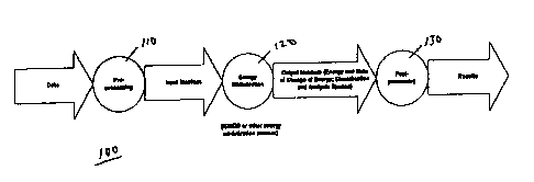
Referring now to FIG. 1, it illustrates an operational block diagram of a
data analysis/classifier tool 100. The least energy deformation
analyzer/classifier
is a three-step process. Step 110 is a front end for data transformation. Step
120
is a process step implementing energy minimization and deformation
computations-in the presently preferred embodiment, this process step is
implemented through the IDMDS algorithm. Step 130 is a back end which
CA 02315814 2000-06-21
WO 99/34316 PCT/US98/27374
interprets or decodes the output of the process step 120. These three steps
are
illustrated in FIG. 1.
It is to be understood that the steps forming the tool 100 may be
implemented in a computer usable medium or in a computer system as computer
5 executable software code. In such an embodiment, step 110 may be configured
as
a code, step 120 may be configured as second code and step 120 may be
configured as third code, with each code comprising a plurality of machine
readable steps or operations for performing the specified operations. While
step
110, step 120 and step 130 have been shown as three separate elements, their
10 functionality can be combined and/or distributed. It is to be further
understood
that "medium" is intended to broadly include any suitable medium, including
analog or digital, hardware or software, now in use or developed in the
future.
Step 110 of the tool 100 is the transformation of the data into matrix form.
The only constraint on this transformation for the illustrated embodiment is
that
the resulting matrices be square. The type of transformation used depends on
the
data to be processed and the goal of the analysis. In particular, it is not
required
that the matrices be proximity matrices in the traditional sense associated
with
IDMDS. For example, time series and other sequential data may be transformed
into source matrices through straight substitution into entries of symmetric
matrices of sufficient dimensionality (this transformation will be discussed
in
more detail in an example below). Time series or other signal processing data
may also be Fourier or otherwise analyzed and then transformed to matrix form.
Step 120 of the tool 100 implements energy minimization and extraction of
deformation information through IDNIDS. In the IDMDS embodiment of the tool
100, the stress function Q defines an energy functional over configurations
and
transformations. The configurations are further restricted to those which
satisfy
the constraint equations Xk = ZWk . For each configuration Xk , the weight
vectors diag( Wk ) are the contextual signature, with respect to the common
space,
of the k th input source. Interpretation of o~ as an energy functional is
CA 02315814 2000-06-21
WO 99/34316 PCT/US98/27374
11
fundamental; it greatly expands the applicability of MDS as an energy
minimization engine for data classification and analysis.
Step 130 consists of both visual and analytic methods for decoding and
interpreting the source space W from step 120. Unlike traditional applications
of
IDMDS, tool 100 often produces high dimensional output. Among other things,
this makes visual interpretation and decoding of the source space problematic.
Possible analytic methods for understanding the high dimensional spaces
include,
but are not limited to, linear programming techniques for hyperplane and
decision
surface estimation, cluster analysis techniques, and generalized gravitational
model computations. A source space dye-dropping or tracer technique has been
developed for both source space visualization and analytic postprocessing.
Step
130 may also consist in recording stress/energy, or the rate of change of
stress/energy, over multiple dimensions. The graph of energy (rate or change
or
stress/energy) against dimension can be used to determine network and
dynamical
system dimensionality. The graph of stress/energy against dimensionality is
traditionally called a scree plot. The use and purpose of the scree plot is
greatly
extended in the present embodiment of the tool 100.
Let S = {Sk } be a collection of data sets or sources Sk for k =1, . . ., m .
Step 110 of the tool 100 converts each Sk E S to matrix form M(Sk ) where
M(Sk ) is a p dimensional real hollow symmetric matrix. Hollow means the
diagonal entries of M(Sk ) are zero. As indicated above, M(Sk ) need not be
symmetric or hollow, but for simplicity of exposition these additional
restrictions
are adopted. Note also that the matrix dimensionality p is a function of the
data S
and the goal of the analysis. Since M(Sk ) is hollow symmetric, it can be
interpreted and processed in IDMDS as a proximity (dissimilarity) matrix. Step
110 can be represented by the map
M:S--~Hp(R),
Sk H M(Sk )
CA 02315814 2000-06-21
WO 99/34316 PCT/US98/27374
12
where H p (R) is the set of p dimensional hollow real symmetric matrices. The
precise rule for computing Mdepends on the type of data in S, and the purpose
of
the analysis. For example, if S contains time series data, then M might entail
the
straightforward entry-wise encoding mentioned above. If S consists of optical
character recognition data, or some other kind of geometric data, then M(Sk )
may
be a standard distance matrix whose ij-th entry is the Euclidean distance
between
"on" pixels i and j. M can also be combined with other transformations to form
the composite, (M o F)(Sk ) , where F, for example, is a fast Fourier
transform
(FFT) on signal data Sk . To make this more concrete, in the examples below M
will be explicitly calculated in a number of different ways. It should also be
pointed out that for certain data collections S it is possible to analyze the
conjugate
or transpose S' of S. For instance, in data mining applications, it is useful
to
transpose records (clients) and fields {client attributes) thus allowing
analysis of
attributes as well as clients. The mapping M is simply applied to the
transposed
data.
Step 120 of the presently preferred embodiment of the tool 100 is the
application of IDMDS to the set of input matrices M{S) _ {M(Sk )} . Each
M(Sk ) E M(S) is an input source for IDMDS. As described above, the IDMDS
output is a common space Z c R" and a source space W. The dimensionality n of
these spaces depends on the input data S and the goal of the analysis. For
signal
data, it is often useful to set n = p -1 or even n = I Sk ~ where ISk ~
denotes the
cardinality of Sk . For data compression, low dimensional output spaces are
essential. In the case of network reconstruction, system dimensionality is
discovered by the invention itself.
IDMDS can be thought of as a constrained energy minimization process.
As discussed above,the stress Q is an energy functional defined over
transformations and configurations in R" ; the constraints are defined by the
constraint equation Xk = ZWk . IDIVIDS attempts to find the lowest stress or
energy configurations Xk which also satisfy the constraint equation. (MDS is
the
CA 02315814 2000-06-21
WO 99/34316 PCT/US98/27374
13
special case when each Wk = l ,the identity matrix.) Configurations Xk most
similar to the source matrices M(Sk ) have the lowest energy. At the same
time,
each Xk is required to match the common space Z up to deformation defined by
the weight matrices Wk . The common space serves as a characteristic, or
reference object. Differences between individual configurations are expressed
in
terms of this characteristic object with these differences encoded in the
weight
matrices Wk . The deformation information contained in the weight matrices,
or,
equivalently, in the weight vectors defined by their diagonal entries, becomes
the
signature of the configurations Xk and hence the sources Sk (through M(Sk ) ).
The source space may be thought of as a signature classification space.
The weight space signatures are contextual; they are defined with respect to
the reference object Z. The contextual nature of the source deformation
signature
is fundamental. As the polygon classification example below will show, Z-
contextuality of the signature allows the tool 100 to display integrated
unsupervised machine learning and generalization. The analyzer/classifier
learns
seamlessly and invisibly. Z contextuality also allows the tool 100 to operate
without a priori data models. The analyzer/classifier constructs its own model
of
the data, the common space Z.
Step 130, the back end of the tool 100, decodes and interprets the source or
classification space output W from IDIvIDS. Since this output can be high
dimensional, visualization techniques must be supplemented by analytic methods
of interpretation. A dye-dropping or tracer technique has been developed for
both
visual and analytic postprocessing. This entails differential marking or
coloring of
source space output. The specification of the dye-dropping is contingent upon
the
data and overall analysis goals. For example, dye-dropping may be two-color or
binary allowing separating hyperplanes to be visually or analytically
determined.
For an analytic approach to separating hyperplanes using binary dye-dropping
see
Bosch, R. and Smith, J, "Separating hyperplanes and the authorship of the
disputed federalist papers," American Mathematical Monthly, Vol. 105, 1998.
CA 02315814 2000-06-21
WO 99/34316 PCT/US98/27374
14
Discrete dye-dropping, allows the definition of generalized gravitational
clustering
measures of the form
xA(x) exp(p ~ d (x, y))
g (A, x) = y"x
exp( p ~ d (x, y))
yxx
Here, A denotes a subset of W {indicated by dye-dropping), xA(x), is the
characteristic function on A, d (~,~) is a distance function, and p E R . Such
measures may be useful for estimating missing values in data bases. Dye-
dropping can be defined continuously, as well, producing a kind of height
function
on W. This allows the definition of decision surfaces or volumetric
discriminators.
The source space W is also analyzable using standard cluster analytic
techniques.
The precise clustering metric depends on the specifications and conditions of
the
IDMDS analysis in question.
Finally, as mentioned earlier, the stress/energy and rate of change of
stress/energy can be used as postprocessing tools. Minima or kinks in a plot
of
energy, or the rate of change of energy, over dimension can be used to
determine
the dimensionality of complex networks and general dynamical systems for which
only partial output information is available. In fact, this technique allows
dimensionality to be inferred often from only a single data stream of time
series of
observed data.
A number of examples are presented below to illustrate the method and
apparatus in accordance with the present invention. These examples are
illustrative only and in no way limit the scope of the method or apparatus.
Example A: Classi tcation o~f regular ~no~,~ons
The goal of this experiment was to classify a set of regular polygons. The
collection S = {S, , . . . , S,6 } with data sets S, - S4 , equilateral
triangles; SS - Sg ,
squares; S9 - S,Z , pentagons; and S~3 - S,6 ; hexagons. Within each subset of
distinct polygons, the size of the figures is increasing with the subscript.
The
perimeter of each polygon Sk was divided into 60 equal segments with the
CA 02315814 2000-06-21
WO 99/34316 PCTIUS98/27374
segment endpoints ordered clockwise from a fixed initial endpoint. A turtle
application was then applied to each polygon to compute the Euclidean distance
from each segment endpoint to every other segment endpoint (initial endpoint
included). Let xst denote the i-th endpoint of polygon Sk , then the mapping M
is
5 defined by
M:S~H6°(R),
Sk H (dsk i dsk ~ . . . ~ d~ j
where the columns
dst =(d(xs,~xsk)~d(xs,~xsx)~...,d(xst,xs°))'.
The individual column vectors d~; have intrinsic interest. When plotted as
functions of arc length they represent a geometric signal which contains both
frequency and spatial information.
The 16, 60 x 60 distance matrices were input into a publicly distributed
version of PROXSCAL. PROXSCAL was run with the following technical
specifications: sources- 16, objects- 60, dimension- 4, model- weighted,
initial
configuration- Torgerson, conditionality- unconditional, transformations-
numerical, rate of convergence- 0.0, number of iterations- 500, and minimum
stress- 0Ø
FIG. 2 and FIG. 3 show the four dimensional common and source space
output. The common space configuration appears to be a multifaceted
representation of the original polygons. It forms a simple closed path in four
dimensions which, when viewed from different angles, or, what is essentially
the
same thing, when deformed by the weight matrices, produces a best, in the
sense
of minimal energy, representation of each of the two dimensional polygonal
CA 02315814 2000-06-21
W O 99/34316
16
PCTlUS98/27374
figures. The most successful such representation appears to be that of the
triangle
projected onto the plane determined by dimensions 2 and 4.
In the source space, the different types of polygons are arranged, and
hence, classified, along different radii. Magnitudes within each such radial
$ classification indicate polygon size or scale with the smaller polygons
located
nearer the origin.
The contextual nature of the polygon classification is embodied in the
common space configuration. Intuitively, this configuration looks like a
single,
carefully bent wire loop. When viewed from different angles, as encoded by the
source space vectors, this loop of wire looks variously like a triangle, a
square, a
pentagon, or a hexagon.
Example B' Classif cation of non-reQUlar polvgons
The polygons in Example A were regular. In this example, irregular
polygons S = {5,,...,S6} are considered, where S, - S3 are triangles and S4 -
S6
rectangles. The perimeter of each figure Sk was divided into 30 equal segments
with the preprocessing transformation M computed as in Example A. This
produced 6, 30 x 30 source matrices which were input into PROXSCAL with
technical specifications the same as those above except for the number of
sources,
6, and objects, 30.
FIG. 4 and FIG. S show the three dimensional common and source space
outputs. The common space configuration, again, has a "holographic" or faceted
quality; when illuminated from different angles, it represents each of the
polygonal
figures. As before, this change of viewpoint is encoded in the source space
weight
vectors. While the weight vectors encoding triangles and rectangles are no
longer
radially arranged, they can clearly be separated by a hyperplane and are thus
accurately classified by the analysis tool as presently embodied.
It is notable that two dimensional IDMDS outputs were not sufficient to
classify these polygons in the sense that source space separating hyperplanes
did
not exist in two dimensions.
CA 02315814 2000-06-21
WO 99/34316
17
PCT/US98/27374
E_xamDle C.' Time series data
This example relates to signal processing and demonstrates the analysis
tool's invariance with respect to phase and frequency modification of time
series
data. It also demonstrates an entry-wise approach to computing the
preprocessing
transformation M.
The set S = {S,,...,5,2} consisted of sine, square, and sawtooth waveforms.
Four versions of each waveform were included, each modified for frequency and
phase content. Indices 1-4 indicate sine, 5-8 square, and 9-12 sawtooth
frequency
and phase modified waveforms. All signals had unit amplitude and were sampled
at 32 equal intervals x, for 0 s x s 2~r .
Each time series Sk was mapped into a symmetric matrix as follows. First,
an "empty" nine dimensional, lower triangular matrix Tk = (t~ ) = T(Sk ) was
created. "Empty" meant that Tk had no entries below the diagonal and zeros
everywhere else. Nine dimensions were chosen since nine is the smallest
positive
integer m satisfying the inequality m(m -1) l 2 >_ 32 and m(m -1) l 2 is the
number
of entries below the diagonal in an m dimensional matrix. The empty entries in
Tk were then filled in, from upper left to lower right, column by column, by
reading in the time series data from Sk . Explicitly: s; = t2, , the first
sample in Sk
was written in the second row, first column of Tk ; sz = t3, ,the second
sample in
Sk was written in the third row, first column of Tk , and so on. Since there
were
only 32 signal samples for 36 empty slots in Tk , the four remaining entries
were
designated missing by writing -2 in these positions (These entries are then
ignored
when calculating the stress). Finally, a hollow symmetric matrix was defined
by
setting
M(Sk ) = Tk + Tk' .
This preprocessing produced 12, 9 x 9 source matrices which were input to
PROXSCAL with the following technical specifications: sources- 12, objects- 9,
CA 02315814 2000-06-21
W O 99/34316
18
PCT/US98127374
dimension- 8, model- weighted, initial configuration- Torgerson,
conditionality-
unconditional, transformations- ordinal, approach to ties- secondary, rate of
convergence- 0.0, number of iterations- 500, and minimum stress- 0Ø Note
that
the data, while metric or numeric, was transformed as if it were ordinal or
S nonmetric. The use of nonmetric IDMDS has been greatly extended in the
present
embodiment of the tool 100.
FIG. 6 shows the eight dimensional source space output for the time series
data. The projection in dimensions seven and eight, as detailed in FIG. 7,
shows
the input signals are separated by hyperplanes into sine, square, and sawtooth
waveform classes independent of the frequency or phase content of the signals.
Example D' SeauenceJ Fibonacci. etc.
The data set S = {5,,...,S9 } in this example consisted of nine sequences
with ten elements each; they are shown in Table 1, FIG. 8. Sequences 1-3 are
constant, arithmetic, and Fibonacci sequences respectively. Sequences 4-6 are
these same sequences with some error or noise introduced. Sequences 7-9 are
the
same as 1-3, but the negative 1's indicate that these elements are missing or
unknown.
The nine source matrices M(Sk ) _ (m J ) were defined by
m~~ = I Sk - $i
the absolute value of the difference of the i-th and j-th elements in sequence
Sk .
The resulting 10 x 10 source matrices where input to PROXSCAL configured as
follows: sources- 9, objects- 10, dimension- 8, model- weighted, initial
configuration- simplex, conditionality- unconditional, transformations-
numerical,
rate of convergence- 0.0, number of iterations- 500, and minimum stress- 0Ø
FIG. 9 shows dimensions 5 and 6 of the eight dimensional source space
output. The sequences are clustered, hence classified, according to whether
they
are constant, arithmetic, or Fibonacci based. Note that in this projection,
the
constant sequence and the constant sequence with missing element coincide,
CA 02315814 2000-06-21
WO 99/34316 PCTNS98/27374
19
therefore only two versions of the constant sequence are visible. This result
demonstrates that the tool 100 of the presently preferred embodiment can
function
on noisy or error containing, partially known, sequential data sets.
Example E: Missin~v_alue estimation for bridges
This example extends the previous result to demonstrate the applicability of
the analysis tool to missing value estimation on noisy, real-world data. The
data
set consisted of nine categories of bridge data from the National Bridge
Inventory
(NBI) of the Federal Highway Administration. One of these categories, bridge
material (steel or concrete), was removed from the database. The goal was to
repopulate this missing category using the technique of the presently
preferred
embodiment to estimate the missing values.
One hundred bridges were arbitrarily chosen from the NBI. Each bridge
defined an eight dimensional vector of data with components the NBI
categories.
These vectors were preprocessed as in Example D, creating one hundred 8 x 8
source matrices. The matrices were submitted to PROXSCAL with specifications:
sources- 100, objects- 8, dimension- 7, model- weighted, initial configuration-
simplex, conditionality- unconditional, transformations- numerical, rate of
convergence- 0.0, number of iterations- 500, and minimum stress- 0.00001.
The seven dimensional source space output was partially labeled by bridge
material-an application of dye-dropping-and analyzed using the following
function
~.f~, (x) ~ d (x~ y)-v
gP (Al' x) = y~x
d (x~ Y)-P
ysx
where p is an empirically determined negative number, d (x, y) is Euclidean
distance on the source space, and x,~ is the characteristic function on
material set
A; , i =1,2 , where A, is steel, Az concrete. (For the bridge data, no two
bridges
had the same source space coordinates, hence gP was well-defined.) A bridge
CA 02315814 2000-06-21
WO 99/34316 PCT/US98/27374
was determined to be steel (concrete) ifgP(A"x) > gp(AZ,x)
( g p ( A, , x ) < g p ( AZ , x) ). The result was indeterminate in case of
equality.
The tool 100 illustrated in FIG. 1 estimated bridge construction material
with 90 percent accuracy.
5 Example F: Network dimensionalit~,for a 4-node network
This example demonstrates the use of stress/energy minima to determine
network dimensionality from partial network output data. Dimensionality, in
this
example, means the number of nodes in a network.
A four-node network was constructed as follows: generator nodes 1 to 3
10 were defined by the sine functions, sin(2x), sin( 2x + 2 ) , and sin( 2x +
43 ) ; node 4
was the sum of nodes 1 through 3. The output of node 4 was sampled at 32 equal
intervals between 0 and 2~r .
The data from node 4 was preprocessed in the manner of Example D: the
ij-th entry of the source matrix for node 4 was defined to be the absolute
value of
15 the difference between the i-th and j-th samples of the node 4 time series.
A
second, reference, source matrix was defined using the same preprocessing
technique, now applied to thirty two equal interval samples of the function
sin(x)
for 0 S x S 2~r . The resulting 2, 32 x 32 source matrices were input to
PROXSCAL with technical specification: sources- 2, objects- 32, dimension- 1
to
20 ~ 6, model- weighted, initial configuration- simplex, conditionality-
conditional,
transformations- numerical, rate of convergence- 0.0, number of iterations-
500,
and minimum stress- 0Ø The dimension specification had a range of values, 1
to
6. The dimension resulting in the lowest stress/energy is the dimensionality
of the
underlying network.
Table 2, FIG. 10, shows dimension and corresponding stress/energy values
from the analysis by the tool 100 of the 4-node network. The stress/energy
minimum is achieved in dimension 4, hence the tool 100 has correctly
determined
network dimensionality. Similar experiments were run with more sophisticated
dynamical systems and networks. Each of these experiments resulted in the
successful determination of system degrees of freedom or dimensionality. These
CA 02315814 2000-06-21
WO 99/34316 PCT/US98/27374
21
experiments included the determination of the dimensionality of a linear
feedback
shift register. These devices generate pseudo-random bit streams and are
designed
to conceal their dimensionality.
From the foregoing, it can be seen that the illustrated embodiment of the
present invention provides a method and apparatus for classifying input data.
Input data are received and formed into one or more matrices. The matrices are
processed using IDMDS to produce a stress/energy value, a rate or change of
stress/energy value, a source space and a common space. An output or back end
process uses analytical or visual methods to interpret the source space and
the
common space. The technique in accordance with the present invention therefore
avoids limitations associated with statistical pattern recognition techniques,
which
are limited to detecting only the expected statistical pattern, and
syntactical pattern
recognition techniques, which cannot perceive beyond the expected structures.
Further, the tool in accordance with the present invention is not limited to
the
fixed structure of neural pattern recognizers. The technique in accordance
with the
present invention locates patterns in data without interference from
preconceptions
of models or users about the data. The pattern recognition method in
accordance
with the present invention uses energy minimization to allow data to self
organize,
causing structure to emerge. Furthermore, the technique in accordance with the
.present invention determines the dimension of dynamical systems from partial
data streams measured on those systems through calculation of stress/energy or
rate of change of stress/energy across dimensions.
While a particular embodiment of the present invention has been shown
and described, modifications may be made. For example, PROXSCAL may be
replaced by other IDMDS routines which are commercially available or are
proprietary. It is therefore intended in the appended claims to cover all such
changes and modifications which fall within the true spirit and scope of the
invention.
CA 02315814 2000-06-21
WO 99/34316 PCT/US98/Z7374
22
ENERGY MINIMIZATION ~'PENDIX
FOR
CLASSIFICATION, PATTERN RECOGNITION,
SENSOR FUSION, DATA COMPRESSION,
NETWORK RECONSTRUCTION, AND SIGNAL PROCESSING
SOURCE CODE FOR PRESENTLY PREFERRED EMBODIMENT OF THE INVENTION
(c) 1998 Abel Wolman and Jeff Glickman
STEP 1. PREPROCESSING SnrIRC~ CnnF
Mathematica code for step 1 of the invention: preprocessing.
Mathematica packages:
< < LiaearAlQebra' Matri»laai.Du7.aticm' l
Packages for preprocessing:
(* Creates dissimilarity matrix from list of data vectors. No missiaQ values.
*)
HeQiaPackaQe["MakeDissMat'"]
MakaDissMatssusags =
"DZakeDissMat[M] creates dissiasilarity matrices frcm list of lists M."
BlQia["'Private'"]
MakeDissE~at [t~] s a Module [ {DissMat} ,
DissMat[L ] := Module[(lea . LeaQth[L]},
Table[Abs[Lt till -Lltjlll. {i. lea), ii, lea}]
is
If[MatrixQ[M],
priest["Number of sourcees ", IaaQth[Mll3
print["lsuanber of objectss °, Length[M[ [1] l l l:
Flattaa[DissMat /AM, 1] ,
Priest["Number Of sourcess 1"]j
Priest["N~bar of objectss ", i~az~th[M] ] 1
DisaMat[M]]
1
~Il
Wit]
A1
CA 02315814 2000-06-21
WO 99/34316 PCT/US98/27374
23
(* Creates dissimilarity matrices fz~a~ ratings
data with alternative distaacea and allowance for missing data *)
BegiuPackage [ "D~aksDissMissVal' "]
MakeDiesD~issVals susage =
"MakaDissml.seVal[R,foz~a,metric,mv,prnt] creates (ao. of columns) source
dissimilarity matrices from matrix R with possible missing values. set ms=1 to
i~icate mias3,ng values ms=0 otherwise= metric specifies the distance functi~
to be calculated. R is assumed to have the form: objects-by-categories.
gasses specifications are: fos~l. list of dissimilarity matricest
foraa~2, vector form, a single dissimilarity matrixf fora~3, stacked
dissimilarity matrices. prat=1 means priest source and object count."
Hsgin["'Private'"]
MaksDisaMisaVal[R~, foza~, metric, mv_, prnt_] :_
Nodule[{Rt, m~obj, nsmisource, dissims, vectform, stackform, tamp= 0},
j = [Rl :
=f[i,ength[R[ 11111 == o, Rt a Transpose[neap[Liar, R] ], Rt = Transpose[R] ]
f
numsourca = Length[Rt]f
If [prat == 1,
Print["Number Of Sources: ", numsource]t
Print["Ntmlber Of ObjeCtsi ", nlmbbj]]J
dissims a Table[Table[If [ (Rt[ [k, i] ] < o p Rt[ [k, j] ] < o) &aan. sa 1 &a
i != j, -1, Which[
metric == 1, If [ (tai = Abs [Rt [ [k, i] ] - Rt [ [k, j ] ] ] ) > 10" (-5) .
tamq~, 0] , metric == 2,
xf [ (tasqp = Log[Aba [Rt [ [k, i] ] - Rt [ [k, j 111 + il ) > to ~ (-5) ,
tai, o] , True, o] ] ,
{i, a~obj}, {j, aumobj}], {k, numaource}] f
vectform=Table[sort[(R[[i]] -R[[j]]) ~ (R[[ill -R[Ijll)1. {i, numobj}, (j,
numobj}] j
stackfozm = JoiaoAdissims=
Which[fosm == 1, dissims / / N, form == 2, vectform / / N, form == 3,
stackform / / N]
l:
~[1
E.hdPaclsage [ 1
A2
CA 02315814 2000-06-21
WO 99/34316 PCT/US98/27374
24
(* Creates hybrid dissimilarity matrix *)
8eginPackage["did."]
Needs["LiasarAlgebra'MatriWanipulation'"]f
Needs["MakeDissNissVal'"]f
(* need to use this package since need -1 in border of matrix *)
F~rbrid::usage .
"hybrid[L] creates hyrbrid dissimilarity matrices from list of data vectors
L."
Begin[~'PriVate'"]
F~id[L_] s=Module[{output, toprorovs, restofrows},
tOpr09ns a Map[{JOin[{0}, #] }&, L] f
restofrows s Map~readi~,p~peadRC~Og(#1, #a]&,
{Map[Traaapose[{#}]&, L], MakeDissMissVal[Transpose[L], 1, 1, 1, 0]}]f
output = Flatten[Ma~pThread[Join[#1, #a]&, {toprooos, restofroovs} ] , 1] f
print["Dh>mber Of saurcess ", Length[L]];
print("Number of objects: ", Length[output[[1]]]]f
output
]
~I]
EadPackage[]
A3
CA 02315814 2000-06-21
WO 99/34316 PCT/US98/Z7374
(* Creates Toanlitz proximity matrices *)
BsQinPacIsaQe["MakeToeplitz'"]
MnkeToeplitzs:usaQe .
"MakeToepiitz[L] creates a Toaplitz proacimity matrix from the list L."
HeQiu [ "' Pritrate' " j
MakeToaplitz(M ] s= Module({Toeplitz},
Toeplitz[L_] s= Module((len = Length[L], size},
size = 1+ len (lea- 1) / 2=
For(i ~ 1, i <= size, i++,
P'or[ j = 1, j <= size, j++,
If[i== j, a[i, j] s 0.0, a[i, j] =LI[Abs[i- j]]]]
]s
]t
Table[a[i, j], Vii, size}, {j, size}]
J:
If[MatrixQ(M],
Print["I~er Of s0llrCesi ", ~th[M]}~
Print["Number of ~objectss ", Leu~th[M[[1]]] + 1]f
flatten[Toeplitz/eM, 1],
Print["Number of ~saurcsas 1"]f
Print["Number Of objectss ", LeaQth(M] + 1]f
Toeplitz[M]]
1
EadPackaye[}
A4
CA 02315814 2000-06-21
WO 99/34316 PCT/US98/27374
26
(* Creates proximity matrices by populating symmetric matrix of appropriate
size *)
HegissPackage[~MakeSymMat~"]
MaxeSymMat::usage =
"MakeSymMat[M] creates a sst of Symmetric matrices fzroaa the list of data
vectors M
through entsywise substitution into a symmetric matrix of appropriate size."
Begin["Private'"]
MaxeSya~lat [l~] : = Module [ { } ,
Print["~mbsr of souraas: ". Leagth[M]]t
sya:[Y_] : s MOdule [ {autaiat = { } , symlen = Length[v] , x z 1, symsize} ,
symaize = (Sqrt [8 symlen+ 1] + 1) / 2 f
For[i = 1, i <= symsize, i++,
For[ j =1, j < i, j++,
a[i, j] =v[[x}] f a[j, i] =v[[x}}, x++,
It
Js
Table[=f[i== j, 0, a[i, j]], {i, symsize}, {j, symsize}]
It
Augment [L ] : = Module [ (auglea, n, taanp} ,
auglen a heaflth[L]f
n = auglenf
teak = 1 f
While[2auglen-n"2-n<=0, tee=n+1=n--]f
Flatten[Join[L, Table[-1, { (tee (teak - 1) / 2) - auglen} ] ] ]
l:
outmat = Flatten[Map[syat[Augment[#] 1 ~. M] , 1]:
priest["I~hm:ber of objects: ~, Length[outmat[ [1} ] ] ] r
autmat
I
~[1
~dPackage[]
AS
CA 02315814 2000-06-21
WO 99/34316 PCT/US98/Z7374
27
(* Creates distance matrices fran sets of configurations of pouts *)
8eginPaCkage["Lp~"]
Lpssusage = "Lp[C, p] calulates Miakoro~ski
distance avith e>~onent p on eats C of configuratiams of points."
Begin["Private'"]
Lp[C_, p ] :. Module[(metric},
metric[X_, a_] := Module[{len ~ Length[x]},
(Partition[PlusAATranspose[
Flatten[Table[Abs[(X[[i]] -xllj]])] "a. {i, lan}, {j, lan}], 1]], lan]) "
(i/a) //
N
]f
Zf[MatrixQ[C[[1]]].
Print["Nvmnbar of sources: ". l~ngthlC]If
Print["Number of objects: ", Length[C[[1]]]]~
Flatten[rsap [metric [#, p] &, c] , 1] ,
Print["Number of sources: 1"];
Print["N~nber of objects: ", Length[C]]=
metric[C, p]]
]
~Il
EodPackaga[]
(* Output fross preprocessing packages *)
Print["Test data: "]~
teat = {{1, 2, 3}, {1, 5, 9]}=
test / / Tablegorm
Print["MakeDissMat output on test data:"]~
MakeDissbtat[test] // TablaFOrm
Print["MakeDisaMissVal output on test Batas"]
MakeDissMissVal[Transpose[test], 3, 1, 1, 1] // TableForm
Print["Fi~brid output an test data:"]
F~rbrid[test] // TableFOrm
print["NakeToeplitz output oan test data:"]
MakeToeplitz[test] // TableForm
Print["MakeBymMat output On test data:"]
MakeBya~lHat [ test] / / TableForm
Print["Lp output on test data:"]
Lp[teat, 2] // TableFozm
Test data:
1 2 3
1 5 9
MakeDissMat output on test data:
Number of sources: 2
A6
CA 02315814 2000-06-21
WO 99!34316 PCT/US98/27374
28
Number of objects: 3
0 1 2
1 0 1
2 1 0
0 4 8
4 0 4
8 4 0
MakeDiasMissVal output on test data:
Number of sources: 2
Number of objects: 3
0 1. 2.
1. 0 1.
2. 1. 0
0 4. 8.
4. 0 4.
8. 4. 0
Hybrid output on test data:
Number of sources: 2
Number of objects: 4
0 1 2 3
1 0 1. 2.
2 1. 0 1.
3 2. 1. 0
0 1 5 9
1 0 4. 8.
4. 0 4.
9 8. 4. 0
MakeToeplitz output on test data:
Number of sources: 2
Number of objects: 9
0. 1 2 3
1 0. 1 2
2 1 0. 1
3 2 1 0.
0. 1 5 9
1 0. 1 5
5 1 0. 1
9 5 1 0.
MakeSymMat output on test data:
Number of sources: 2
Number of objects: 3
A7
CA 02315814 2000-06-21
WO 99l3431G PCT/US98/27374
29
0 1 2
1 0 3
2 3 0
0 1 5
1 0 9
9 0
Lp output on test data:
Number of sources: 1
Number of objects: 2
A8
CA 02315814 2000-06-21
WO 99/34316 PCT/US98/27374
0 6.7082
6.7082 0
STEP 2. PRO IN ~,ILrRC~ CODE
Mathematica code for step 2 of the invention: processing.
Mathematica code for IDMDS via Alternating Least Squares and Singular Value
Decomposition.
IDMDS via Alternating Least Squares (ALS)
Mathematica packages:
< < LinearAlgebra' Choleslq~' f
« Graphics'Graphics3D'f
« Graphics'Graphics'f
« Graphics'MultipleListPlot'f
Subpackages for TDMDS via ALS:
(* distance matrix package *)
BaginPackage["?matrix'"]
Ltnatrix: :usage =
"ianatrix[C] calculates the Lh:clidean iuterpoint distances o! input
configuration C."
Begin["'Private'"]
ixnatrix[C_] sa Module[{numobj},
at>mobj = hngth[C] f
Table(Sqrt[(C[[i]] -C[[j]]) ~ (C[[i]] -C([j]])], {i, m>mobj}, {j, numobj}] //N
l
~tl
E~BPackage[]
(* Stress Package *)
BegiaPackage["Stress'"]
Nesds["Nmatrix'"]f
Stress:: usage = "Stress[P,W,X] calculates Rruskal's stress."
Begin["'Private'"]
Stress[P_, W_, X_] :-- Module[{},
PlusA~Flatten[ (Map[W* #&, P] -Map[bnatrix, X] ) "2]
]
Wit]
EndPackage[]
A9
CA 02315814 2000-06-21
WO 99/34316 PCT/US98/27374
31
( * Ciuttmaa Package * )
BeQiIlPaCkagA ( "(~ttttfi~IS' " ]
Needs(~Dmatrix'~]f
f~uttaiaas s usage =
"Cauttman[P,X,W] ca~utes the update co~sfiQuratia~n via the Quttman
transfoxm.~
Hegiu["'Private'"]
Ciuttman [ P , X , W_] s -- Module [ { 8, D. d, dim} ,
D = Dmatrix[X] f
d1m a Length(X] f
d a Le>zgth(8] f
8 = Table
xf[i m j ~~ D([i, ill is o. -(Wf(i, jll * p((i, jll) /D((i, jll~ o], {i, d},
{j, d}lf
N[ (1 / dim} * (B - 8lan[DiagossalMatrix[8 [ [i] ] ] , {i, d} ] ) . X]
1
~(1
EadPackage[]
(* Vlnat Package *]
HaginPackage[~VMat'"]
VMats:usage a ~VMatjW] coa~utes the p.s.d. V matrix fraan the areight matrix
W."
Begin("'PriVat~'~]
VMat [W ] i= btodule ( {dial a Length[W] , V},
VaTable(=f(i !a j, -W((i~ j]l~ ~]~ {i, dial}, {j, disR}] f
V + siml(DiagoualMatrix( (-1) * V [ [i] ] ] , {i, dim} ]
J
~(l
E~sdPackage [ ]
(* UnitNozm Package *)
HeginPackage[~UnitNozm'"]
thiitNorsns :usage a ~VaitNoxm(A] takes the
list of diagonals A sad uait nornializes thaan so that ( 1/n) ~1~A~ 1. "
Begin("'Private'"]
UaitNorm[A_] s= Module({},
Map[84rt(Plus~ (A~2) ] " (-1) * #&, A] * Sqrt[Length[A] ] // N
1
~(]
EladPackage [ ]
A10
CA 02315814 2000-06-21
WO 99/34316 PCT/US98/27374
32
(* That Package *)
HAQinPaCkaQe[~TMat~~]
TMats susage a ~~at[A] defines the T matrix which noxmalizes castmoas specs
Z."
HaQia["'Private'~]
That [A ] : ~ bZodula [ { } .
DiaQoaalMatrix[sart(pluseo (A" 2) ] * ( (sit[i,enQth[A] ] ) " (-1) ) ] // N
]
P~sd [ ]
EndPackaQe(]
(* InitialConfig Package *)
BeQiaPackaQe["InitialConfiQ'"]
ZnitialConfigssueaQe = "?ssitialCanfiQ[sas, no, d] creates nsanumber of
sources, ao=
number of objects by d-dimensional constraiaed randaan start configurations."
Begin["'Private'"]
InitialConfig(ns_. no_, d_] s=
MOdule ( {numBOUrC~8 a ns, numObB a n0, di~i8 a d, i, j, k, Q, w} ,
a = N(Table( (*seedRaadasn(i* j] J*)Raadom[], {i, ~msobs}. { j, dimsms} ] l J
w = N[Table[(*BeedRandom[k*j]J*)Rsadcm(], {k, numsaurces}, {j, dim~ss}I]J
{Table[a.DiaQonalMatrix(w[(k]]], {k, numaources}}, d, w}
1
~I]
EodPackaQe[]
(* Diagonal Package *)
HaQinPackags(~DiaQonal'~]
DiaQonalssusaQe a ~DiaQonal[M] creates a diagonal matrix from main diagonal of
M."
HeQin["'Private'"]
Diagonal[M_] := Module[{dim},
dim - LeaQth(M] J
Table(If[is= j, M([i, j]], 0]. {i, dim}. {j. dim}] //N
}
~I]
EndPackage[}
All
CA 02315814 2000-06-21
WO 99/34316 PCT/US98/27374
33
( * UaDiagox:al Package * )
BeginPackage[ "ZfiDiagoa:al' "]
UnDiagonal::usage = "UriDiagonal[M] turns diagonal matrix into a vector."
Begin["'Private'"]
tlnDiagonal [b~] : a Module [ {dim} ,
~ _ [M] f
Table[M[[i, i]], {i, dim)] //N
]
~L]
FasdPackaga [ ]
IDMDS via ALS:
(* IDMDS via ALS *)
BegiaPackage["ID~~SALS'"]
Needs("Stress'"]f
Needs["InitialConfig'"]f
Needs ( "VnitNozai " ] f
[n~t'n]f
NledB("TMat'"]f
Needs("Outtmaa'"]f
Needs("Diagoasal'"]f
Needs [ "Vt:Diagonal' "] f
IDMDSAL3: : usage = "IDMDSALB (prox-, pmxrats_. diaL., epsilon,.,,
itaratioas_,saed_] caa~utes Ids for proad,mity matrices pra~c."
Begin["'Private'"]
IDdmSALS [prox_, pravcoots_, dim_, epsilon , itsratiaus_, sead_] : = Module [
{Aconstrain, A0, BX, deltaatress, deltastreaslist, rnanits, aumobj, aumscs,
stresslist,
T, T0, tem~BtreBS, tes~stressprev, V, Vin, Xupdate, X0, Zconstrain, Zt, ZO},
~j = (D~([1]]]f
aumscs = Length[prox]f
numi.ts a O f
SeedRaadaan( seed] f
{X0, Z0, A0} = InitialCaafig[asanscs, samobj, dim] f
Print["Nuomber of sources: ", numscs]f
Print["Nvm~bar of objects: ", aumobj]f
TO a That[AO] f
ZOnorrn a ZO . TO f
AOnorm a Map ( Inverse [ TO ] . #&, Map [ DiagonalNiatrix, AO ] ] f
XO a Map ( ZOnozat . #&, AOaorm] f
V = VMat[proxwts]f
V~ a PsaudOIx~7CSe ( V] f
tempstrass a Stress[prox, proxwts, XO]f
etresslist a {te~8tress} f
deltastress a tea~stressf
deltastresslist a {}f
A12
CA 02315814 2000-06-21
WO 99/34316 PCT/US98/27374
34
While[deltastress > epsilon&&nutnits <= iterations,
numits++j
7dspdata = MapThrsad[Guttaiaa[#1, #2, pznocwts] &, {praac, XO} ] ;
For[i = 1, i <= 1, i++,
Zcanstraia = ( 1 / asanscs) * (Vt:~ . PluseoMapTlsread[#1 . #2&, {asmaobj *
Xl~pBate, AOnorm} ] ) ;
zt = Transpose[ZCanstraia];
Aconstraia = Map [ Imrerse [Diagonal [ zt . v . Zcanstrain] ] . #&,
Map [Diagonal, Map [Zt . #&, nunabj * Xupdate] ] ] ;
T = TMat(Mnp[VnDiagonal, Acanstrain]];
AOnorm = Map [ I~nerse [T] . #&, Aconstraia] ;
z0noza: = zconstrain . T;
];
XO = Map [ZOnorm . #&, AOnoxm] ;
t1~78tres8~ren = tei~stres8;
taanpstress = Stress [prox, Draxw~ts, XO] ;
stresslist = Append[stresslist, temnpstrese] ;
deltastress = te~stressprev- tes~stresa;
deitastresslist = Appead[daltastresslist, deltastress];
]i
Print["Final stress isi ", tea~stress];
i~rint["Stress record is: ", stresslist];
Print["stress differencess ", deltastreaslist];
Priest [ "Dhm:ber of iterations: ", numits] ;
Print["The caa~on space coordinates are: ", ZOaorm// Matri~ozm];
Print["The source space cooz~iinates are: ". Map[MatrixForm,
Chop[ACOnstrain]]];
{zOnorm, Chop[Aconstraia]}
]
~Il
EodPackage[]
IDMDS via Singular Value Decomposition (SVD)
Mathematica packages:
« Graphics'Graphics3D';
<< Graphics'Graphics';
Subpackages for IDMDS via SVD:
A]3
CA 02315814 2000-06-21
WO 99/34316 PCTNS98/27374
(* DistaaceMatrix Package *)
BegiaPackage["DistanceMatrix'"]
DistaacaMatrix:susage = "DistanceMatrix[
coasfiQ] prcduces~a distance matrix fraus coafiguratian matrix config."
Begin["'private'"]
Dista.caMatrix[confiQ ] := Module[{c, d, m, one, tamp},
d = Length[config]s
m = config . Transpose[config];
c s {Table(m([i, i]], {i, d}]}f
one = {Table[l, {i, d}]};
N [ Sqrt [ Transpose [ one] . c + Tra:sspoas [ c ] . one - 2 m] ]
]
~(l
Et>s~PacxaQa [ l
(* DiaqMatNozas Package *)
Begiapackage["DiagMatNorai ~]
DiagMatNormssusage = "DiagMatNozsn[A] normalizes the list of weight vectors
A."
Begin["'Private'"]
DiagMatNoras[A_List] s= Module[ {neovA, nozsn, suasnorm= 0},
newA = Table(0, {Length[A]}, {Length[A[[1]]]}];
FOr[i a 1, i <= LO~Lgth(A( [1] ] ] , i++,
!~'Or[j = 1, j <a I,~th(A], j++,
sua~,oxm+=A[(~, i]] ~2f
It
norm ( i ] = Scp-t [ sumuorm] t
sussm;oras s 0l
]f
norm = Table[norm[k], {k, Length[A([1]]]}]t
FOr(i = 1, i <a Lsngth(A[ [1] ] ] , i++,
FOr [ j = 1, j < a Z,ength (A] , j ++,
newA[[j, i]] ~A[[j, i]] /norm[[i]]i
1s
]t
N(nerorA]
1
~(J
EndPackage[]
A]4
CA 02315814 2000-06-21
WO 99/34316 PCT/US98/27374
36
( * NoxmalizeC~ * )
HagiaPackage["Normaliza0'"]
Normalizaf3s susage = "Noxa~alizeG[A] gives matrix
which normalizes the case space given the list of weight vectors A."
Begin("'Private'"]
NozmalizeG[A_List] s= G?odule[ {newA, norm, suna~orsn a 0},
szeavA = Table[0, {Lsagth[A] }, {hangth[A[ [1] ] ] } ] j
For[i = 1, i <= Liength[A( [1] ] ] , i++,
For ( j = 1, j <= Length[A] , j++,
sussasoxm+a A( [ j, i] ] "2t
Js
ILO( i] a 8qrt [ s1~10rE1] )
suaaroan = 0 i
]J
noun = Table [norm[k] , {k, Length[A [ [ 1] I l } ] s
N[Diagoxsa7.Nlatrix[noras] ]
]
~I]
E~d.Package [
(* HMatrix Package *)
HeginFaCkage["BNatriX'"]
HMatrixssusage = "BMatrix(delta, DM] is part of the Outtman traasfoass."
Begin ( ° ' Pritlate' " ]
HMatr3x [ delta_, Dl~] s = Module ( {b, bdiag, d, i, j , k} ,
d = Length[delta]f
b = Table[0, {d}, {d}] // Nf
FOr[1 = 1, i <a d, i++,
For[j = 1, j <~ d, j++,
If(i la j && DM[[i, j]] la 0. b((i, j]] = b([i, j]] - delta((i, j]] /I7M[[~.
j]])s
)s
1s
bdiag a g~[Diaganal,Matrix[b[ [k] ] ] , {k, d} ] f
N[b - bdiag]
]
~I]
EndPackage[]
A1 S
CA 02315814 2000-06-21
WO 99/34316 PCT/US98/27374
37
(* Outtms:iTransforrn package *)
HeginPackage["OuttmanTraaeform'"]
OuttmanTraasfozm s s usage = "The Qutt>naaTraaefozsa[B, X]
updates the configuration X through s:nsltiplication by the BMatrix B."
BAgiI1 ( "' Private' "]
OuttmanTraasform[B_, X_] :- Mo~le~(dim},
d~ = i.ezzgthlx] t
1
N~ ~ B.X
EndPackage[]
( * ACiNtBtress Package * )
8egillPaCkage( "AC~IStr~88' "]
Ac~WStress s s usage = "The A(~VStress [dissimilarity,
distaacs] is the loss fuaction for stazltidimensional scaling."
Begin("'Private'"]
ACiWBtress [dissimilarity_, distaace_] s = Module [ ( s, disc, i , j } ,
dim a Length[dissimilarity]j
s s Of
For(j ~ 1, j <= dim, j++,
For(i = 1, i < ~, i++,
s +-_ (dissimilarity[ [ i, ~ 11 - distance [ [ i, j l l ) " 2
]:
]:
N[s]
]
~(I
EndPackage(]
A16
CA 02315814 2000-06-21
WO 99/34316 PCT/US98/27374
38
(* NormBtress *)
BegiaPackage["Normstress'"]
NormStress::usage = "Normstress[dissimilarity] nozmalizes the stress loss
function."
Begin["'Private'"]
Norm9tress[dissimilarity_List] := Dtodule[{noon, numobjacts, i, j},
aumobjacts =Laength[dissimilarity[[1]]];
norm = O . O f
For[j = 1, j <= numobjects, j++,
For[i = 1, i < j, i++,
nozm+-_ dissimilarity[ [i, j] ] "2
]i
]t
N[norm]
]
~[]
EndPackage[]
(* InitialConfig2 Package *)
BegiaPackage["ZnitialConfig2'"]
Initialconfig::usage = "Iaitialconfig[ne, no, d] creates as=rnsober of
sources, no=
number of objects by d-dimensional constraiaed start configurations."
Begin["'private'"]
Initialconfig[ns_, no_, d_] :=
Module[ {numsources a n6, numObB ~ n0, dimen8 = d, i, j, k, d, w},
C3= N[Table[{*seedRaadom[i*j]j*)Raadcm[], (i, numobs}, {j, dimens}]]s
w = N[Table [ (*seedRandcsa[k* j ] ; * ) Random[ ] , {k, numsaurces} . {j.
dues} ] ]
Table[a . Diagonalbiatrix(W [ [k] ] ] , {k, numsaurces} ]
]
~[]
E,hdPackage [ ]
A]7
CA 02315814 2000-06-21
WO 99/34316 PCT/US98/27374
39
(* Torgerson Package *)
BegiaPackage["Torgerson'"]
Torgerson:susage = "Torgeraoa[D, d] caaq~utes classical
2(d) diaisasioaal scaling solution for dissiavilarity matrix D."
Begin["'Private'~]
Torgerson(D_, d~] := Module[ {Dsq, u, v, w, Hdelta, J, One, a = Ireagth[D] },
One = {Table[1, {i, a) ] };
J = IdeatityMatr3x(a] - (1 / a) Transpose[one] . one:
Dsq=N[Map(#~2&, D, 1]];
Hdalta=N[(-0.5) J.Dsq.J];
{u, w, v} . Singulaz'Values(Bdelta, Tolerance-> O];
Transpose[Table[v([i]], {i, d}]].DiagoaalMatrix[Table[w([i]], {i, d}]] // Chop
1
EndPackage(]
(* Ave Package *)
HegiaPackage("Ave'"]
Avessusage = "Ave[M] finds the average of the list of matrices M and
proSuces a list of the same length with every elasreat the average of M."
8lgia("'Private'"]
Ava(M_List] s= Module[{},
average = N [ ( 1 / Length [ M] ) * Apply [ Plus, M] ] _
Table[average, {i, Lexsgth(M] } ]
1
~[]
BSoodPackage [ ]
A18
CA 02315814 2000-06-21
WO 99/34316 PCT/US98/27374
(* SVDConatraiu Package *)
8sgiaPackage["SVDConstraia'"]
SVDConstraiassusage z
"3VDConstrain[configs] isaposes constraints on the list of configurations
configs."
Begin("'Private'"]
SVDCanstraia[configs_List, d_] s= Module[{aumascs = Length[configs],
~mcbjecta = i~ength(confige[ [i] ] ] , dim s d, y, u, v, uhold, vhold, G,
oraights},
For(i = 1, i <= dial, i++,
y[i] a Transpose[Table[Map(Tranepose, coafiga][[k, i]], {k, rnansrcs}]]f
]f Print[Table[y[i], {i, dim}]]f
FOr [ i a 1, i <= dim, i++,
{uhold[i] , w[i] , vhold[i] } = N[8lngulariTalues[Njy[i] ] , Tolerance -> 0]
// Chap] f
]f
a = Table[uhOld[i] , {i, dim} ] ;
v = Table [vhold[i] , {i, dim} ] f
Ci=N[Transpose[Table[u[[i, 1]], {i, dim}]]]f
weights =
N[Partitio~a[~'lattea[Table (w(k] [ [1] ] * v( [k, 1, j 11, { j, aumisrcs},
{k, dim} 11, ~l ] f
Table [ci , btap [DiagonalMatrix, weights] [ [ i ] ] , { i, rnmiarca} ]
]
~[]
EodFackage[]
IDMDS via SVD:
(* ZDI~s via SvD on constraints with implicit normslizaticn of stress. *)
BegiaPackage["IdsddsBVD'"]
Needs["DistaaceMatrix'"]f
Needs("8matrix'"]f
Needs [ "GhsttmauTransfoxsn' "] f
Needs["AOPIBtreas'"]f
Needs ( "NOral$tre9a' "] j
N.eds["DiagmatNosai "]f
Needs["Normalized'"]f
Needs["InitialCoafig2'"]f
Needs["Torgersan'"]f
Needs("SVDCaastraia'"]f
Needs["Ave'"]f
Nseda["C~raphica'oraphics'"]f
Needs["Ciraphics'araphics3D'"];
Idmds3VDssusaga a
"I~Id88VD[
dies, dim, iterations, rata, start] is an IDMn.9 package for an arbitrary
znmiber
of sources. Ester a list of diasia~ilarity matrices = dissf the dimension =
dim of the coassmon spacef the number of iterations required = iterations;
the rate of comr~ergence a rate. Iias raadosn, start=if Torgerson,
A]9
CA 02315814 2000-06-21
WO 99/34316 PCT/US98I27374
41
start=2t or user-provided, start=stastlist start cosifi~uratic~s."
geyin["'Private'"]
IdmdsBVD[diss_, dial, iteratioms_, rate, start] s=
Module ( ~ d a dial, B s rate, d, Ouorm, fit, boldstress, iterate,
kossstaat, aumit = iterations, su~abjects. a~nsrcs = Length[dies] . edr,
sr, stress, strsssdiffrecord, stressrscord, taa~, tetapstress,
u, updates, uta~p, v, vtaa~, o', weiQhtracord, meiyhts, ~eiQhtsnoxsn, wr} ,
rn>mobjects = ~.~th(diss[ (1] } ] f
taa~stress = 0.0=
holdstress = 0.0=
Stress a 0 . 0 f
kcnstaat = 0 . 0 f
iterate = 0 t
For [ i a 1, i <= numsrcs, it+,
konstaat += NossnStress[disa[[i]}1t
]1
xf [I~m~barQ(start] && start a= 1, t~ = IaitialConfiQ2[maosrcs, numobjects, d]
] s
I![NumbarQ(start] && start as 2, teak a SVDConstrai:i[Map(ToxQersaai[#, d]&,
dies] , d] ] s
If [I3~oberQ(start] && start == 3, taa~ a SvDConstrain[Dlap[TorQersou[#, d] &,
Ave [dies] ] , d] ] t
xf [NvmibsrQ(start] _= False, tend = start] t
FOr(i a 1, i <_ ~7~Brcs, i++,
holdstreas += Ac~lBtrase[dies( [i] ] . DistanceMatrix[teak[ [i] ] ]
It
]t
If [><~onstaat ! a 0,
stress a holdstress / kanstaat,
stress = holdatresa] t
Print["Initial stress is: ", stress]s
s9ra (0.0}=
sr = (stress} j
v~z'= (}t
t~ri~sile [ iterate < a a~nit,
FOr(i s 1, i <a ~irCS, it+,
~[i]
OuttmenTraasfoza~(BMstrix[dies [ [i] ] , DistaaceMatrix[taanp( [i] ] ] ] ,
teonp( (i] ] ]
}:
X = Table [Qt [i] , ( i, aaanarcs} ] s
For ( i = 1, i <= d, i++,
Y[i] = Traaapose[Table[Map[Transpose, X] [ [1c, i] ] , (Ic, nutnsrcs} ] ] s
]t
For[i = 1, i <= d, i++,
(uta~[i] . w[i] . vtaae~[i] } = N[S3aagulerValues[y(i] } 1 i
]s
A2~
CA 02315814 2000-06-21
WO 99/34316 PCTlUS98/27374
42
a=Table[ute~[i], {i, d}]t
v s Table[vte~[i], {i, d}] t
ti = N[Transpose[Table[u( [i, 1] ], {i, d}] ] ] t
(*Print("c3 is: ",Matri~es'orm[c3] ] t*)
waighta = N[Partition[Flatten[Table[w[k] [ [1] ] * v[ [k, 1, j] ] , { j,
numsrcs}, {k, d} ] ] , d] ] t
taanp = Table[d . Map[Diagonalblatrix, wai~hts] [ [i] ] , {i, rnanarcs} ] t
tamrpstress = O.Ot
For [ i = I t holdstress = 0 . 0, i < _ na>msrcs, i++,
holdstress +-- A0~8treas [dies [ [i] ] , DiataaceMatrix[tai [ [i] ] ] ] t
]t
If [konstant 1= 0,
temapstrese = holdstress / konatant,
ta~streas = holdstrsss] t
weiQhtrecord = Appa~sdTo [avr, wsi~'hts] t
strasarecord = llppeasdTo [ sr, te~stress] t
stressdiffrecord = AppendTo [ sdr, stress - tempstress ] t
If [stress - tas~pstrsss <= e, Brsak[] ,
stress = t~patresst
iterate++t
] ~ (* end If *)
] t ( * end afbile * )
C~aoxm = o . Noxaializec~(araiQhts] t
areiQhtsnorm = Dia~2stNoz:n[waiQhts] t
For[ j = 1, j <= rn>msrcs, j++,
For(i = 1, i <a d, i++,
If[wei~htsnozm[[j, i]] < 0,
w~siQhtsnoxas= ReplacePart[weiQhtanossn, -wsiShtenorm[ ( j, i] ] , { j, i} ] t
]t
]:
]t
Print["Number of iterations wass ", iterate]t
Print ( "Final itre8s s ", taae~etreas} t
Print("Stress difference records ", stressdiffrecord]t
Print("Stress records ", stressrecord]t
Print("Coordinates of the cameson spaces"]t
Print[Matrix~'orm[cmorm] ] t
Print["Coozdinatea of the wsiQht spaces "]t
Print[MatrixForsn[weiQhtsnorm]]t
(*Print["Coordinates of the private spacess "]t
Print[Map[MatzixForm,Map[Q.#&,Map[Diegotsalblatrix,waiQhtsnoxm]]]]f*)
Print("Plot Of coas~on space:"]t
Which[d == 3, ScatterPlot3D[C~norm, PlotStyle -> ({AbsolutePoiatSize[5]}}],
A2 ]
CA 02315814 2000-06-21
WO 99/34316 PCT/US98/Z7374
43
d sa 2, TeXtLiBtplOt(Qtlo7Gal] , d as 1,
ListPlot [Flatten[G~noxm] , .plotJoined -> True, Axes -> False, Frame -> Txue]
;
It
Priest["Plot of the source spaces"]:
~sich(d a= 3, 8catterPlot3D(weiQhtsnoxm, Plot8tyle ->
{{AbsolutePoint8ize[5]}},
ViewPoiat -> {2.857, 0.884, 1.600}(*,ViewPoiat->{1.377, 1.402, 2.827}*)], d =a
2,
TextListplot[weiQhtsnorsa, PlotRanQa -> A11, Axes -> False, FYame -> True] , d
as l,
ListPlot [Flattaa[weiQhtsaorm] , PlotJoiaed -> Ts~e, Axes -> False, Frame ->
True] f
It
l
~I1
Et~dPackaQe [ ]
STEP 3 POSTPRO IN OURCF ~C'OD~
Mathematica code for step 3 of the invention: postprocessing.
Subfunctions:
(* L~clidsaa distaace between vactors a and v *)
d(u . v_l =a ~'t( (u-v) ~ (u-~11 // N:
(* Characteristic function *)
char[u_, x_] : a If [x aaa u, 1, 0] _
Clustering functions for back-end analysis of classifying space of invention:
Qi[obj_, dy~aval_, dyelist_, Ll_, L2_, ~awer_] :a Plus~Table[If[i as obj, 0,
char[dlreval, dyelist[ [i] ] ] djLi [ [obj] ] , L2 [ [i] ] ] " (poover) ] .
{i. LenQth[dyelist] } ] /
PluaAA
Table[=f [i =a obj, 0, d[L1[ (obj] ] , L2 [ (i] ] 1 " (ewer) 1. {i. LenQth[L2]
} ] t
Q2 [obj_, dyewal_, dyelist_, L2_, powar_] : a PluseATable[If (i -= obj, 0,
char(dyeval, dyelist[ [i] ] ] d[L2 [ [obj) ] , L2 [ [i] ] ] ~ (pororar) ] ,
{i, Length[dyelist] } ] /
PlusAA
Table(If [i as obj, 0, d[L2 ( [obj] ] , L2 ( [i] 11 " (Poe'er) 1 ~ {i~ (~] ? 1
f
st3 l~j_, d~l_, 4~rolist_, L2_, ~c~er ]
Plus~Table[=f [i == obj, 0, char[dyeval, dyeliat( [i] ] ]
E~(d(L2 [ (obj] ] , L2 ( [i] 1 ] 1 " (veer) 1. {i, LenQth[dyelist] } ] /
Plusoe
Table[If(iaaObj, 0, EXp(d(L2((Obj]], L2((i]111 "(D~'>1, {ii LAnQth[L2]}];
A22