Note : Les descriptions sont présentées dans la langue officielle dans laquelle elles ont été soumises.
CA 02499476 2005-03-18
WO 2004/030022 PCT/CA2003/001318
Automated Optimization of Asymmetric Waveform Generator LC Tuning
Electronics
Field of the Invention
[001] The instant invention relates generally to high field asymmetric
waveform
ion mobility spectrometry (FAIMS), more particularly the instant invention
relates to
a method of optimizing asymmetric waveform generator LC tuning electronics.
Background of the Invention
[002] High sensitivity and amenability to miniaturization for field-portable
applications have helped to make ion mobility spectrometry (IMS) an important
technique for the detection of many compounds, including narcotics,
explosives, and
chemical warfare agents as described, for example, by G. Eiceman and Z. Karpas
in
their book entitled "Ion Mobility Spectrometry" (CRC, Boca Raton, 1994). In
IMS,
gas-phase ion mobilities are determined using a drift tube with a constant
electric
field. Ions are separated in the drift tube on the basis of differences in
their drift
velocities. At low electric field strength, for example 200 V/cm, the drift
velocity of
an ion is proportional to the applied electric field strength, and the
mobility, K, which
is determined from experimentation, is independent of the applied electric
field.
Additionally, in IMS the ions travel through a bath gas that is at
sufficiently high
pressure that the ions rapidly reach constant velocity when driven by the
force of an
electric field that is constant both in time and location. This is to be
clearly
distinguished from those techniques, most of which are related to mass
spectrometry,
in which the gas pressure is sufficiently low that, if under the influence of
a constant
electric field, the ions continue to accelerate.
[003] E.A. Mason and E.W. McDaniel in their book entitled "Transport
Properties
of Ions in Gases" (Wiley, New York, 1988) teach that at high electric field
strength,
for instance fields stronger than approximately 5,000 V/cm, the ion drift
velocity is no
longer directly proportional to the applied electric field, and K is better
represented by
KH, a non-constant high field mobility term. The dependence of KH on the
applied
electric field has been the basis for the development of high field asymmetric
waveform ion mobility spectrometry (FAIMS). Ions are separated in FAIMS on the
CA 02499476 2005-03-18
WO 2004/030022 PCT/CA2003/001318
basis of a difference in the mobility of an ion at high field strength, KH,
relative to the
mobility of the ion at low field strength, K. In other words, the ions are
separated due
to the compound dependent behavior of KH as a function of the applied electric
field
strength.
[004] In general, a device for separating ions according to the FAIMS
principle
has an analyzer region that is defined by a space between first and second
spaced-
apart electrodes. The first electrode is maintained at a selected do voltage,
often at
ground potential, while the second electrode has an asymmetric waveform V (t)
applied to it. The asymmetric waveform V(t) is composed of a repeating pattern
including a high voltage component, VH, lasting for a short period of time tH
and a
lower voltage component, VL, of opposite polarity, lasting a longer period of
time tL.
The waveform is synthesized such that the integrated voltage-time product, and
thus
the field-time product, applied to the second electrode during each complete
cycle of
the waveform is zero, for instance VH tH + VL tL = 0; for example +2000 V for
10 ~,s
followed by -1000 V for 20 ~,s. The peak voltage during the shorter, high
voltage
portion of the waveform is called the "dispersion voltage" or DV, which is
identically
referred to as the applied asymmetric waveform voltage.
[005] Generally, the ions that are to be separated are entrained in a stream
of gas
flowing through the FAIMS analyzer region, for example between a pair of
horizontally oriented, spaced-apart electrodes. Accordingly, the net motion of
an ion
within the analyzer region is the sum of a horizontal x-axis component due to
the
stream of gas and a transverse y-axis component due to the applied electric
field.
During the high voltage portion of the waveform an ion moves with a y-axis
velocity
component given by vH = KHEH, where EH is the applied field, and KH is the
high field
ion mobility under operating electric field, pressure and temperature
conditions. The
distance traveled by the ion during the high voltage portion of the waveforrn
is given
by dH = vHtH = KHEHtH, where tH is the time period of the applied high
voltage.
During the longer duration, opposite polarity, low voltage portion of the
asymmetric
waveform, the y-axis velocity component of the ion is vL = KEL, where K is the
low
field ion mobility under operating pressure and temperature conditions. The
distance
traveled is dL = VLtL = KELtL. Since the asymmetric waveform ensures that (VH
tH) +
(VL tL) = 0, the field-time products EHtH and ELtL are equal in magnitude.
Thus, if KH
2
CA 02499476 2005-03-18
WO 2004/030022 PCT/CA2003/001318
and K are identical, dH and dL are equal, and the ion is returned to its
original position
along the y-axis during the negative cycle of the waveform. If at EH the
mobility KH >
K, the ion experiences a net displacement from its original position relative
to the y-
axis. For example, if a positive ion travels farther during the positive
portion of the
waveform, for instance dH > dL, then the ion migrates away from the second
electrode
and eventually will be neutralized at tk~e first electrode.
[006] In order to reverse the transverse drift of the positive ion in the
above
example, a constant negative do voltage is applied to the second electrode.
The
difference between the do voltage that is applied to the first electrode and
the do
voltage that is applied to the second electrode is called the "compensation
voltage"
(CV). The CV voltage prevents the ion from migrating toward either the second
or
the first electrode. If ions derived from two compounds respond differently to
the
applied high strength electric fields, the ratio of KH to K may be different
for each
compound. Consequently, the magnitude of the CV that is necessary to prevent
the
drift of the ion toward either electrode is also different for each compound.
Thus,
when a mixture including several species of ions, each with a unique KH/K
ratio, is
being analyzed by FAIMS, only one species of ion is selectively transmitted to
a
detector for a given combination of CV and DV. In one type of FAIMS
experiment,
the applied CV is scanned with time, for instance the CV is slowly ramped or
optionally the CV is stepped from one voltage to a next voltage, and a
resulting
intensity of transmitted ions is measured. In this way a CV spectrum showing
the
total ion current as a function of CV, is obtained.
[007] In FAIMS, the optimum dispersion voltage waveform for obtaining the
maximum possible ion detection sensitivity on a per cycle basis takes the
shape of an
asymmetric square wave with a zero time-averaged value. In practice this
asymmetric
square waveform is difficult to produce and apply to the FAIMS electrodes
because of
electrical power consumption considerations. For example, without a tuned
circuit
the power P which would be required to drive a capacitive load of capacitance
C, at
frequency f, with a peak voltage V, is 2~VzfC. Accordingly, if a square wave
at 750
kHz, 4000 V peak voltage is applied to a 20 picofarad load, the power
consumption
will be 240 Watts. If, on the other hand, a waveform is applied via a tuned
circuit, the
power consumption is reduced to P(cos0) where O is the angle between the
current
3
CA 02499476 2005-03-18
WO 2004/030022 PCT/CA2003/001318
and the voltage applied to the capacitive load. This power consumption
approaches
zero if the current and voltage are out of phase by 90 degrees, as they would
be in a
perfectly tuned LC circuit.
[008] Since a tuned circuit cannot provide a square wave, an approximation of
a
square wave is taken as the first terms of a Fourier series expansion. One
possible
approach is to use:
V (t) = 3 D sin(wt) + 3 D sin(2wt - ~c / 2) (1)
Where V(t) is the asymmetric waveform voltage as a function of time, D is the
peak
voltage (defined as dispersion voltage DV), ev is the waveform frequency in
radians/sec. The first term is a sinusoidal wave at frequency co, and the
second term is
a sinusoidal wave at double the frequency of the first sinusoidal wave, 2r.~.
The
second term could also be represented as a cosine, without the phase shift of
~/2.
[009] In practice, both the optimization of the LC tuning and maintenance of
the
exact amplitude of the first and second applied sinusoidal waves and the phase
angle
between the two waves is required to achieve long term, stable operation of a
FAIMS
system powered by such an asymmetric waveform generator. Accordingly, feedback
control is required to ensure that the output signal is stable and that the
correct
waveform shape is maintained.
[0010] In United States Patent 5,801,379, which was issued on September 1,
1998,
Kouznetsov teaches a high voltage waveform generator having separate phase
correction and amplitude correction circuits. 'This system uses additional
hardware
components in the separate phase correction and amplitude correction circuits,
thereby increasing complexity and increasing the cost of manufacturing and
testing
the devices. Furthermore, this system cannot be implemented into control
software,
making it difficult to vary certain parameters.
[0011] It is an object of the instant invention to provide a method of
optimizing
asymmetric waveform generator LC tuning electronics that overcomes the
limitations
of the prior art.
4
kHz, 4000 V peak voltage is app
CA 02499476 2005-03-18
WO 2004/030022 PCT/CA2003/001318
Summary of the Invention
[0012] In accordance with an aspect of the instant invention there is provided
a
method of controlling an asymmetric waveform generated as a combination of a
plurality of sinusoidal waves including two sinusoidal waves having a
frequency that
differs by a factor of two, the method comprising the steps of: sampling the
generated
asymmetric waveform to obtain a set of data points that is indicative of the
generated
asymmetric waveform; normalizing each data point of the set of data points;
determining at least a value relating to the normalized data points; comparing
the
determined at least a value to template data relating to an ideal asymmetric
waveform;
and, in dependence upon the comparison, effecting a change to the generated
asymmetric waveform.
[0013] In accordance with another aspect of the instant invention there is
provided a
method of controlling an asymmetric waveform generated as a combination of a
plurality of sinusoidal waves including two sinusoidal waves having a
frequency that
differs by a factor of two, the method comprising the steps of: sampling the
generated
asymmetric waveform to determine a plurality of data points from a plurality
of
different cycles of the generated asymmetric waveform, the plurality of data
points
being indicative of a shape of the generated asymmetric waveform; analyzing
the
plurality of data points indicative of a shape of the generated asymmetric
waveform,
the step of analyzing being performed other than in dependence upon an order
of
magnitude of the data points; and, in dependence upon the step of analyzing,
effecting
a change to the generated asymmetric waveform.
[0014] In accordance with still another aspect of the instant invention there
is
provided a storage medium encoded with machine-readable computer program code
for controlling an asymmetric waveform generated as a combination of a
plurality of
sinusoidal waves including two sinusoidal waves having a frequency that
differs by a
factor of two, the storage medium including instructions for: obtaining a set
of data
points that is indicative of the generated asymmetric waveform; normalizing
the data
points of the set of data points; applying a predetermined function to the
normalized
data points of the set of data points, to determine a set of resultant values
including
one resultant value corresponding to each normalized data point of the set of
CA 02499476 2005-03-18
WO 2004/030022 PCT/CA2003/001318
normalized data points; determining at least a value relating to the set of
resultant
values; comparing the determined at least a value to template data relating to
an ideal
asymmetric waveform; and, in dependence upon the comparison, adjusting at
least
one of a phase angle difference between the two sinusoidal waves and an
amplitude of
at least one of the two sinusoidal waves.
Brief Description of the Drawings
[0015] Exemplary embodiments of the invention will now be described in
conjunction with the following drawings, in which similar reference numbers
designate similar items:
[0016] Figure 1 shows a plurality of cycles of an asymmetric waveform that is
formed as a combination of first and second sinusoidal waves of frequency ~
and 2~,
respectively;
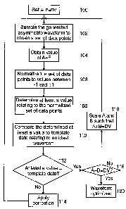
[0017] Figure 2 is a simplified flow diagram of a method of optimizing
asymmetric
waveform generator LC tuning electronics according to an embodiment of the
instant
invention;
[0018] Figure 3 is a simplified flow diagram of a method of applying a
correction at
step 114 of Figure 2 according to an embodiment of the instant invention; and,
[0019] Figure 4 is a simplified flow diagram of another method of applying a
correction at step 114 of Figure 2 according to an embodiment of the instant
invention.
Detailed Description of the Drawings
[0020] The following description is presented to enable a person skilled in
the art to
make and use the invention, and is provided in the context of a particular
application
and its requirements. Various modifications to the disclosed embodiments will
be
readily apparent to those skilled in the art, and the general principles
defined herein
may be applied to other embodiments and applications without departing from
the
spirit and the scope of the invention. Thus, the present invention is not
intended to be
6
CA 02499476 2005-03-18
WO 2004/030022 PCT/CA2003/001318
limited to the embodiments disclosed, but is to be accorded the widest scope
consistent with the principles and features disclosed herein.
[0021] As is noted above, the waveform applied in FAIMS is a combination of
two
sinusoidal waves of frequency r.~ and 2co. The two waves are of.amplitudes
that differ
by a factor of two and are also offset by a phase angle (O), resulting in a
waveform
that is defined by, for example, Equation 2, below:
V (t) = A sin(~t) +B sin(2c~t - O) (2)
where V (t) is the asymmetric waveform voltage as a function of time, A is the
amplitude of the first sinusoidal wave at frequency cv, where a~ is the
frequency in
radians/sec, and B is the amplitude of the second sinusoidal wave at a
frequency 2cv.
This second sinusoidal wave is offset from the first by a phase angle O, which
preferably is equal to ~/2. In practice, the CV is often applied to the same
electrode as
the asymmetric waveform and this do offset is added to V(t) in Equation 2.
[0022] Using the approach of Equation 1, in a waveform having an optimum
shape,
A = 2B, and O is equal to ~ /2. The electroiuc circuit maintains these two
conditions
in order to achieve the waveform with the correct asymmetric waveform shape
for
stable performance of a FAIMS system attached thereto. In a related function,
the
peak voltage on the highest voltage side of the asymmetric waveform (defined
as DV
above) is constant, and equal to A+B. The electronic circuit therefore tracks,
modifies
and controls three parameters, namely A, B and O while simultaneously ensuring
that
A = 2B and that A+B equals the dispersion voltage (DV). Also, the waveform
voltage at the dip in the waveform on the opposite polarity from DV is equal
to A-B.
[0023] Referring to Figure 1, shown is a plurality of cycles of an ideal
asymmetric
waveform that is formed as a combination of first and second sinusoidal waves
of
frequency cv and 2cv, respectively. The asymmetric waveform shape shown in
Figure
1 can for example be established by collecting sample data points from the
waveform,
such as by analog-to-digital (A/D) sampling, in order to acquire a
representative set of
data points from all portions of the asymmetric waveform. The A/D data points
are
optionally taken randomly, at frequencies that are higher than or lower than
the
waveform itself. However, it is necessary that this array of data points of
the signal
7
CA 02499476 2005-03-18
WO 2004/030022 PCT/CA2003/001318
intensity of the asymmetric waveform correctly represent all time periods
within the
waveform. For example, the sample data points should include points near the
peak
voltage 2 in the polarity of maximum voltage applied, as well as points near
the two
peaks 4 of maximum voltage at the other polarity and in the dip 6 between the
two
peaks 4. If the waveform is sampled across all times, the series of points
thus
acquired can be subjected to simple tests to determine if the waveform shape
is
optimum.
[0024] The values of A and B are taken so that, in the instant example, A+B=1
and
AB=2. The peak values 2 of the waveform are therefore equal to A+B. The
opposite
polarity part of the waveform, negative polarity in this example, is
characterized by a
dip 6 and two peak values 4. The value at dip 6 is A-B (in this case A-B=1/3),
and the
peaks 4 in the opposite polarity are each (A+B)/2 (in this case (A+B)/2 =
1/2).
[0025] Three specific types of deviation from the ideal asymmetric waveform
are
possible: first, a phase shift error; second an error in the ratio of AB
(keeping
A+B=1); and third, an error in the sum of A+B (keeping the ratio AB = 2). The
electronics of a not illustrated asymmetric waveform generator must be able to
identify such deviations from the ideal waveform shape, and make adjustments
to the
drive electronics accordingly. In the instant method, it is assumed that A+B
is set to
the desired value, and accordingly the third type of error is corrected
independently of
the other two types of errors.
[0026] Referring now to Figure 2, shown is a simplified flow diagram of a
method
of optimizing asymmetric waveform generator LC tuning electronics according to
an
embodiment of the instant invention. At optional step 100, the sum of the
amplitudes
of the two sinusoidal waves, A+B, is set to a predetermined value, for
instance,
A+B=DV. At step 102 the generated asymmetric waveform is sampled to obtain a
set
of data points. For example, step 102 is performed as a fast analog-to-digital
sampling (A/D) of the waveform voltage to collect 100 data points within one
cycle of
the waveform. A plot of the magnitude, or A/D values, of these data points as
a
function of time of collection yields a trace that resembles an oscilloscope
trace of the
original generated asymmetric waveform. Alternatively, the set of data points
is
obtained as a slow, random, sampling version of A/D, which eventually collects
8
CA 02499476 2005-03-18
WO 2004/030022 PCT/CA2003/001318
sample data points from every portion of the generated asymmetric waveform.
For
example, the A/D collection of 100 data points randomly, one new data point
each
millisecond, results in the acquisition of the 100 data points in
approximately 100
milliseconds. Since the asymmetric waveform is repeating rapidly, perhaps in
the
megahertz range, no two of these A/D data points is sampled from the same
cycle of
the waveform. However, each data point is sampled from somewhere during the
cycle of the waveform. Similarly, each one of the following ninety-nine data
points is
sampled from a random point in a widely separated (in time) cycle of the
waveform,
relative to the previous data point. If the data points are actually random,
then every
region of the generated asymmetric waveform, given the finite number of data
points
collected, is sampled although one does not know from which time in the period
of
the generated asymmetric waveform each data point is acquired. One cannot
reconstruct the equivalent of an oscilloscope trace of the original waveform
shape
because the "time" values of the data points relative to the original waveform
is
unknown, hence the randomness of this sampling method.
[0027] At step 104, the value of A+B is obtained. For example, the set of data
points is provided to a processor having stored therein computer readable
program
code for processing the set of data points according to a predetermined
process. For
example, the value of A+B is found by searching for the largest absolute
magnitude
(most positive or most negative) data point in the set of data points. At step
106, the
data points are normalized. That is to say, after the value of A+B is
obtained, all of
the points are divided by the absolute magnitude value, so that all data
points fall
between -1 and +1.
[0028] At step 108, at least a value relating to the normalized set of data
points is
determined. For example, the set of data points is provided to a processor
having
stored therein computer readable program code for processing the set of data
points
according to a predetermined process. In order to facilitate a better
understanding of
the instant invention, step 108 will be discussed in greater detail by way of
a specific
and non-limiting example in which a value relating to an average of the cubed
value
of the individual data points of the set of data points ("average of the
cubes") is
determined. For example, if the A/D normalized result is 0.4, then 0.4 cubed
is 0.4
times 0.4 times 0.4 equals 0.064. In this example -1 cubed is of course equal
to -1,
9
CA 02499476 2005-03-18
WO 2004/030022 PCT/CA2003/001318
and -0.2 cubed is equal to -0.008. These examples are given to avoid
misunderstanding of this extremely simple process. In addition, the sign of
the result
is important. The average of the cubed value of the normalized data points is
taken as
the sum of the cubes divided by the number of normalized data points. The
average is
not dependent upon the number of data points collected, unless the number of
data
points is too small. Of course, the sum of the cubed values could be used as
an
alternative to the "average of the cubes." Use of the sum gives a value that
depends
upon the number of data points collected. In addition, use of other functions,
including squares, will be discussed in greater detail, below.
[0029] The "average of the cubes" reaches a maximum absolute value when the
asymmetric waveform is optimized. For example, when DV of an ideal asymmetric
waveform is positive, the "average of the cubes" of the normalized waveform is
also
positive and equal to approximately +0.111. When the DV is negative the
"average of
the cubes" is negative and equal to approximately -0.111. In each case, if the
phase
angle offset between the two sinusoidal waves is changed from the optimum
value of
~/2, then the "average of the cubes" begins to deviate towards zero, i.e. the
absolute
value of the "average of the cubes" decreases. Similarly, if the relative
ratio of A/B
deviates from the optimum value of 2, the "average of the cubes" also
deviates.
towards zero. .
[0030] In the process using the "average of the cubes", the objective of the
electronic control circuit and computer code is therefore to adjust the values
of A, B
and the phase angle to maximize, with the correct sign, the value of the
"average of
the cubes." At this maximum of the "average of the cubes", the normalized
positive
polarity asymmetric waveform is shaped in the way that is shown in Figure 1.
Accordingly, at step 110 the determined at least a value is compared to
template data
relating to the ideal waveform. In the instant example, where the polarity of
the DV is
positive, the template data relating to the ideal waveform is a single value,
namely
approximately +0.111.
[0031] At decision step 112, it is determined whether the at least a value is
equal to
the template data relating to the ideal waveform. If the answer at decision
step 112 is
yes, then the shape of the generated asymmetric waveform is optimized to the
ideal
CA 02499476 2005-03-18
WO 2004/030022 PCT/CA2003/001318
shape; however, the absolute magnitudes of the two sinusoidal waves may be
incorrect. Accordingly, at decision step 116 it is determined whether the
value of
A+B is equal to DV. If the answer at decision step 116 is no, then at step 118
the
values of A and B are scaled in the appropriate direction, keeping the ratio
A/B
constant, such that the condition A+B=DV is satisfied. If the answer at
decision step
116 is yes, then the waveform is considered at step 120 to be optimized.
[0032] If the answer at decision step 112 is no, then the shape of the
generated
asymmetric waveform is likely not optimized, and corrective action is required
at step
114. Typically, applying a correction to the generated asymmetric waveform
involves
adjusting at least one of the phase angle offset between the two sinusoidal
waves (O),
and the relative magnitudes of the two sinusoidal waves (A/B). Steps 102 to
112 are
then repeated.
[0033] Once the generated asymmetric waveform is optimized, re-optimization is
carried out, for example, at times dependent on the expected drift rates in
the
amplitudes of the sinusoidal waves and expected drifts in phase angles that
may be
related to operating temperature, etc.
[0034] Referring now to Figure 3, shown is a simplified flow diagram of a
method
of optimization of the shape of an asymmetric waveform, with positive DV,
according
to an embodiment of the instant invention. At decision step 130, it is
determined
whether the at least a value, in this case the "average of the cubes", is
equal to zero. If
the answer at decision step 130 is yes, then at decision step 132 it is
determined
whether both input wave circuits are functioning correctly. For example, if
the output
of the waveform generator is sinusoidal, as would be the case when one of the
two
input sinusoidal waves is zero, then modification of the phase angle offset or
the
relative amplitudes of the input waves cannot change the "average of the
cubes" to a
non-zero value. If the "average of the cubes" is zero, both input sinusoidal
waves are
set to a predefined value, without concern about the particular ratio of A/B.
If the
"average of the cubes" remains at zero, then a failure of one of the two input
waves is
possible. If under these conditions the phase angle offset is changed and the
"average
of the cubes" continues to be fixed at zero, failure of one of the input waves
is certain
and an error is registered at step 134. If it is determined at step 132 that
both input
11
CA 02499476 2005-03-18
WO 2004/030022 PCT/CA2003/001318
wave circuits are functioning correctly, then the amplitudes of the two
sinusoidal
waveforms are set to predetermined values at step 136, and optimization of the
generated asymmetric waveform shape continues.
[0035] After ensuring that the two sinusoidal waves are functional, the
"average of
the cubes" is maximized by adjusting the phase angle offset between the two
sinusoidal waves. For instance, at step 138 the phase angle offset is adjusted
to effect
a change to the shape of the generated asymmetric waveform. At step 140, the
generated asymmetric waveform is sampled in a manner similar to that described
above with reference to Figure 2. A set of data points acquired at step 140 is
normalized at step 142, and a new at least a value is determined relating to
the
normalized set of data points of the adjusted waveform at step 144. At step
146 it is
determined whether the new at least a value is at a maximum value. For
example, this
is done in an iterative manner until additional changes to the phase angle
offset result
in a decrease to the new at least a value. Note that the maximum value at this
stage
may be a value other than +0.111.
[0036] Following maximization of the "average of the cubes" by adjusting the
phase angle offset, the relative amplitudes of the two sinusoidal waves are
modified.
The amplitude of each sinusoidal wave is increased and decreased to ascertain
the
direction of change necessary to maximize the "average of the cubes." For
example,
at step 148 the ratio AB is adjusted. At step 150, the generated asymmetric
waveform is sampled in a manner similar to that described above with reference
to
Figure 2. A set of data points acquired at step 150 is normalized at step 152,
and a
new at least a value is determined relating to the normalized set of data
points of the
adjusted waveform is determined at step 154. At step 156 it is determined
whether
the new at least a value is at a maximum value. For example, this is done in
an
iterative manner until additional changes to the ratio AB results in a
decrease to the
new at least a value. Again, note that the maximum value at this stage rnay be
a value
other than +0.111.
[0037] If it is determined at decision step 158 that the new at least a value
is equal
to the template data, which in this case is +0.111, then the corrective action
is
complete. However, if the new at least a value is different than the template
data,
12
CA 02499476 2005-03-18
WO 2004/030022 PCT/CA2003/001318
then at step 138 the phase angle offset is again changed until the average of
the cubes
is maximized, etc. This cyclic process continues until the "average of the
cubes"
converges to 0.111.
[0038] Referring now to Figure 4, shown is a simplified flow diagram of
another
method of optimizing the shape of a positive polarity waveform according to an
embodiment of the instant invention. At decision step 130, it is determined
whether
the at least a value, in this case the "average of the cubes", is equal to
zero. If the
answer at decision step 130 is yes, then at decision step 132 it is determined
whether
both input wave circuits are functioning correctly. By way of explanation, if
the
output of the waveform generator is sinusoidal, as would be the case when one
of the
two input sinusoidal waves is zero, then modification of the phase angle
offset or the
relative amplitudes of the input waves cannot change the "average of the
cubes" to a
non-zero value. For example, it at step 132 the "average of the cubes" is
zero, both
input sinusoidal waves are set to a predefined value, without concern about
the
particular ratio of AB. If the "average of the cubes" remains at zero, then a
failure of
one of the two input waves is possible. If under these conditions the phase
angle
offset is changed and the "average of the cubes" continues to be fixed at
zero, failure
of one of the input waves is certain and an error is registered at step 134.
If it is
determined at step 132 that both input wave circuits are functioning
correctly, then the
amplitudes of the two sinusoidal waveforms are set to non-zero values at step
136,
and optimization of the generated asymmetric waveform shape continues.
[0039] After ensuring significant amplitudes of the two sinusoidal waves, the
relative amplitudes of the two sinusoidal waves are modified. The amplitude of
each
sinusoidal wave is increased and decreased to ascertain the direction of
change
necessary to maximize the "average of the cubes." For example, at step 148 the
ratio
A/B is adjusted. At step 150, the generated asymmetric waveform is sampled in
a
manner similar to that described above with reference to Figure 2. A set of
data
points acquired at step 150 is normalized at step 152, and a new at least a
value is
determined relating to the normalized set of data points of the adjusted
waveform is
determined at step 154. At step 156 it is determined whether the new at least
a value
is at a maximum value. For example, this is done in an iterative manner until
13
CA 02499476 2005-03-18
WO 2004/030022 PCT/CA2003/001318
additional changes to the ratio AB results in a decrease to the new at least a
value.
Note that the maximum value at this stage may be a value other than +0.111.
[0040] Following maximization of the "average of the cubes" by adjusting the.
relative amplitudes of the two sinusoidal waves, the phase angle offset
between the
two sinusoidal waves is adjusted. For instance, at step 138 the phase angle
offset is
adjusted to effect a change to the shape of the generated asymmetric waveform.
At
step 140, the generated asymmetric waveform is sampled in a manner similar to
that
described above with reference to Figure 2. A set of data points acquired at
step 140
is normalized at step 142, and a new at least a value is determined relating
to the
normalized set of data points of the adjusted waveform at step 144. At step
146 it is
determined whether the new at least a value is at a maximum value. For
example, this
is done in an iterative manner until additional changes to the phase angle
offset result
in a decrease to the new at least a value. Again, note that the maximum value
at this
stage may be a value other than +0.111.
[0041] If it is determined at decision step 158 that the new at least a value
is equal
to the template data, which in this case is +0.111, then the corrective action
is
complete. However, if the new at least a value is different than the template
data,
then the relative amplitudes of the two sinusoidal waves is again changed
until the
average of the cubes is maximized, etc. This cyclic process continues until
the
"average of the cubes" converges to 0.111.
[0042] The method described with reference to Figures 2 to 4 above is
successful
because the absolute value of the voltage of the waveform is significantly
different in
the positive and negative polarity of the ideal asymmetric waveform. Referring
again
to the normalized asymmetric waveform of positive polarity DV shown in Figure
1,
the maxima 2 in the positive polarity are approximately equal to one, whereas
the
most negative points near 4 are approximately equal to negative one-half. The
cube
function, applied to all of the data points, covering all parts of the
waveform, results
in larger valued "cubes" for the points on the higher voltage polarity side of
the
waveform than the points in the opposite polarity. This tends to push the
average of
the cubes in the direction of the polarity of DV. It should be noted that
application of
this process to symmetrical waveforms (such as a sinusoidal wave) results in a
zero
14
CA 02499476 2005-03-18
WO 2004/030022 PCT/CA2003/001318
average of cubes. This is because all points in the positive polarity are
matched by a
point of equal magnitude in the opposite polarity. The cubes of these two
points are
of equal magnitude but of opposite polarity, and therefore the average of
these two
points is zero. This applies to all the points of the waveform, and the net
average of
the cubes of a sinusoidal wave is zero.
[0043] Optionally, another function may be used in place of the cube function.
The
cube function was chosen merely for illustrative purposes because it
automatically
maintains the sign of the data points. For instance, a negative value cubed
remains
negative. The cube function satisfies all the prerequisites for the successful
application of this method, which are described in greater detail below.
[0044] When applied to positive value data points between zero and one the
selected function must be monotonic increasing or decreasing, and preferably
have a
monotonic increasing or decreasing first derivative, respectively. In
addition, the
selected function must either retain the sign of the data points or
consistently apply
the opposite sign to the data points. Finally, the selected function must
result in
magnitudes of calculated points that are the same regardless of the sign of
the data.
The term "odd function" is defined by f(-x) _ -f(x) and has the properties
discussed in
the preceding two sentences. For example, the square function optionally is
used as
long as the calculation enforces the rule that the square of the negative data
points
results in a negative "square." In this case the "modified square" function
squares the
absolute value of the data point, and applies the sign of the original data
point back to
this squared value. Other even polynomial and power functions might have to be
adjusted in like manner to maintain the sign of the original data. In other
words, the
selected function must provide values which distinguish between input points
of
opposite polarity (in sign, but not in magnitude). The square function (x~)
has a
monotonic increasing first derivative (2x) and a positive second derivative
(+2) at all
positive x between zero and one. In this modified square function the
correction for
signs results in the correct derivatives for negative values of x.
[0045] As further clarification of the criteria for selecting a function that
can be
used for optimization of the waveform, we must re-visit some of the
fundamentals of
FAIMS. The discussion in the introduction section of this document considered,
for
CA 02499476 2005-03-18
WO 2004/030022 PCT/CA2003/001318
the sake of simplicity, the operation of a FAIMS with an applied square wave
version
of the asymmetric waveform. We now carry that discussion to more detail. In
general the integral of the waveform voltage (or field) over one cycle is
zero. Using
the terminology of the introduction, EHtH was equal in magnitude (opposite
sign) to
ELtL which were the integrated field-time products for the positive- and
negative-
going parts of the waveform. This generalization also applies to the waveform
described by Equations (1) and (2). Using the terminology of the introduction,
dH and
dL represent the distances traveled by the ion during each polarity part of
the
waveform. More specifically dH and dL are integrals of the motion defined by
KEt
over that part of the waveform. Since the integrals of the field-time
products, Et, are
equal over each polarity of the waveform, the integrals of K over. the
positive and
negative components of the waveform define the relative sizes of dH and dL. In
general, therefore, the net distance traveled by the ion, dH - dL, can be
taken as
proportional to the integral of K(E) over the duration of the waveform. The
"cube"
algorithm described here is equivalent to setting the ion mobility dependence
on field
equal to K(E) = KL (1 + aE3) where a is a constant that depends on the
compound in
question, as well as experimental variables such as the gas composition,
temperature,
pressure etc. The field E is proportional to the voltage applied V (t),
therefore the net
displacement of the ion after one waveform cycle is proportional to the
integral of
K(V(t)3). In other words, the net displacement of the ion after once cycle of
the
waveform is maximized (and CV is therefore maximized) if the waveform has a
shape
V(t) that maximizes the integral of [V(t)]3. This is equivalent to the 'cube'
algorithm
discussed above which uses the "average of the cubes", and which is one of the
functions suggested in this patent application for optimization of the
waveform.
[0046] From the foregoing discussion it becomes clear that obtaining the
maximum
CV for optimum transmission of an ion in FAIMS could be achieved by using the
actual functional dependence of K(E) for the ion in question. If a particular
ion has
mobility that depends on field as K(E) = KL (1 + aE3 ) where a is a constant
as
described above, then if the "cube" algorithm is applied, the waveform
generator will
produce a wave that maximizes the CV of this ion. In general the functional
dependence on field has been written as K(E) = KL (1 + aE2 + [iE4), where KL
is the
mobility at low field (and has no field-dependence). With the application of
the
16
CA 02499476 2005-03-18
WO 2004/030022 PCT/CA2003/001318
asymmetric waveform, we are therefore trying to maximize the value of the
integral
of K(E), which is equivalent to maximizing the integral of K(V(t)), and
equivalent to
maximizing the integral of KL(1 + aV(t)~ + bV(t)ø) over one cycle of the
waveform,
where a and b are proportional to a and [3 respectively, which in turn is
equivalent to
maximizing [aV(t)2 + bV(t)4] over one cycle of the waveform. In practice, this
is
reduced to the following algorithm. The data points of the measured signal
voltages
of the applied asymmetric waveform are normalized. Each point is squared and
multiplied by "a", and also raised to the fourth power and multiplied by "b",
and these
two value are added together. Since this function is "even", where both
positive and
negative input values result in an output value of the same sign, the sign of
the
original data point is then applied to this calculated value. The set of
computed values
from one cycle of the waveform is reduced to one numerical value by addition
of all
the points, or by averaging all the points, or by computing the equivalent of
the
integral of these values over this cycle of the waveform. The waveform
parameters of
phase angle and ratio of AB are then modified in an iterative manner to
maximize the
value of this computed integral for one cycle of the waveform. This procedure
will
result in a waveform that is very similar to, but not necessarily exactly like
that of
equations (1) and (2). In all cases the phase angle will remain exactly ~/2.
The ratio
of AB will vary from 2.0 in order to maximize the CV for the particular ion
that was
used to produce the values of a and (3, or a and b respectively. Consider some
examples applied to a normalized positive polarity waveform V(t): (1) the
average
value of [V(t)]3 will maximize at 0.111 and at this condition AB is 2 and
phase angle
is ~/2, (2) the average value of the correctly signed [V(t)]2 will maximize at
0.0852
when A/B is 1.70 and phase angle is ~/2, (3) the average value of the
correctly signed
[V(t)]4 will maximize at 0.117 when A/B is 2.30 and phase angle is ~/2, and
(4) the
average value of the correctly signed ([V(t)]2-0.3[V(t)]ø) will maximize at
0.051
when A/B=1.61 and the phase angle is ~c/2. This last function was selected
because it
appears to mimic the actual functionality of the ion mobility of some types of
ions at
high electric field strength. Note however that this last function has a
second
derivative that is negative over a small region between zero and one. These
paragraphs of detailed description have been included in this document in
order to
enable a person skilled in the art to exactly understand the scope and
limitations in
selecting functions to be used to optimize the waveform generator, and to show
that
17
CA 02499476 2005-03-18
WO 2004/030022 PCT/CA2003/001318
the 'rules' of the functions regarding signs and derivatives were given above
to enable
a less-skilled individual to select a function that will work with FAIMS. It
is clear
that a wider allowable set of functions is available, beyond the 'rules'
described
above, but a selection of these additional functions requires a complete
understanding
of the operation of FAIMS. These notes are also intended to allow a skilled
individual to select a function that will yield a waveform having extended
advantages,
not limited by the 'rules' outlined above. For more clarity, the function
applied to
processing the optimization of the waveform can be tailored to match the
change in
the mobility of the ion in strong electric fields, and the CV can thus be
maximized.
[0047] From this discussion it is also clear that equation (1) and (2) are not
the only
available equations for the asymmetric waveform, nor are necessarily the
waveforms
that give the maximum CV for a particular compound. For a given compound, the
waveform that yields the highest CV will often provide the best opportunity
for
improvement of the signal to background ratio, improvement of separation from
other
compounds, and for maximizing the signal intensity due to better focusing at
higher
CV. Many benefits of application of asymmetric waveforms tailor-made for
specific
compounds can be expected.
[0048] The cube root function cannot be used, because, although it is
monotonic
increasing (and decreasing in the negative values) and it retains the signs of
the data,
this function does not give a useful average value. In this case the function
(applied
to positive values) does not have a monotonic increasing first derivative
(i.e, it has a
negative second derivative). In this case the derivative of x"(1/3) is
(1/3)x"(-2/3),
thus the derivative is not increasing as the input values are increased and
its second
derivative is negative.
[0049] The logarithm function cannot be used because the magnitudes of the
results
from calculation for the positive and negative points would be different,
i.e., log(x) is
not equal to log(-x), which doesn't exist. Even if this problem is corrected
using the
"modified log function" such that log(-x) is defined to be -log(abs(x)), where
abs(x) is
the absolute value of x, the second derivative of the logarithm function is
negative.
On the other hand the exponential function can be used if the effect of the
sign of the
data point is eliminated. For example, a "modified exponential" function is
defined,
18
CA 02499476 2005-03-18
WO 2004/030022 PCT/CA2003/001318
in which the exponential of the absolute values of the data points are taken,
followed
by an application of the sign of the original data point. In other words, the
function
sgn(x) is defined to give +1 for positive, and -1 for negative values of x,
which allows
a modified exponential function, sgn(x)exp(abs(x)), to be defined, where
abs(x) is the
absolute value of x. The second derivative of this modified exponential is
positive for
positive values of x and negative for negative values of x.
[0050] The functions to be used in this optimization process therefore are not
limited to cube, modified square, modified exponential functions, but rather
all
functions with the appropriate properties including derivatives. The
application of the
above information of applying a function to further analyze data points
permits a
simple process for feedback and control of the asymmetric waveform in FAIMS.
The
electronics of the waveform generator preferably includes a microprocessor
which
processes the output of a fast or slow A/D converter programmed to collect
sufficient
data points to monitor the generated asymmetric waveform. Since the data
points
may be taken randomly, a random distribution may require the collection of a
larger
number of points than a systematic, high frequency A/D with evenly spaced (in
time)
points. The points are processed by the "average of the cubes", or some other
function, method as described above. If the value of this "average of the
cubes" data
processing is lower than the predicted +0.111 for a positive polarity (DV)
waveform
then corrective action is taken.
[0051] Numerous other embodiments may be envisaged without departing from the
spirit and scope of the instant invention.
19