Note : Les descriptions sont présentées dans la langue officielle dans laquelle elles ont été soumises.
CA 02583337 2014-03-21
Electro-optical method for measuring distance
and detecting a non-ideal chirp profile
The invention relates to an electro-optical distance-measuring method
according to the
pre-characterizing clause of Claim 1, an electro-optical distance-measuring
apparatus according
to the pre-characterizing clause of Claim 12 and a computer program product.
In the area of electronic or electro-optical distance measurement, various
principles and
methods are known. The approach consists in transmitting frequency-modulated
electromagnetic
radiation, such as, for example, visible or non-visible laser light, to the
target to be surveyed and
subsequently receiving one or more echoes from back-reflecting objects,
ideally exclusively from
the target to be surveyed. After reception, the optionally superposed echo
signal is superposed
with a mixing signal and the frequency of the signal to be analysed is thus
reduced so that the
apparatus need not be very complex. The mixing can be effected either as a
homodyne method
with the transmitted signal or as a heterodyne method with a periodic, in
particular harmonic
signal of known period. Thus, the methods differ in that mixing is effected
with the transmitted
signal itself or with a harmonic signal having its own frequency. The mixing
serves for
transforming the received signal to a lower frequency. Subsequently, the
transit times and hence
¨ in the case of known propagation velocity of the radiation used ¨ the
distances to the targets to
be surveyed are determined from the resulting signal.
The apparatuses used for implementing these methods usually use a signal
generator as a
chirp generator, which superposes a signal on a radiation source which can be
modulated. In the
optical area, lasers are generally used as radiation sources. In the optical
area, transmission and
reception optical systems are used for emission and reception, respectively a
detector and
receiver with subsequent mixer, AID converter and digital signal processor
being connected
down-circuit of said optical systems.
Usually, a linear frequency-modulated chirp is generated by the signal
generator as signal
s(t):
s(t)=a+b= cos(27c = OW), =c+d=t+e=t2 (1)
1
CA 02583337 2014-03-21
the instantaneous frequency f (t) = d(t) then being a linear function of time:
dt
f (t)= d +2e = t (2)
which simplifies the determination of transit times.
In the case of n targets having relative amplitudes A k and transit times tk
(k = 1, ...,n), the
noise-free echo signal e(t) can be written as follows:
e(t)= EAks(t¨tk) (3)
k =I
This echo signal e(t) is detected and is mixed with the signal m(t):
{
s(t ¨to), homodyne
m(t) = (4)
cos(27-c(fot + (D)), heterodyne
The mixing with m(t) results in the signal
d(t)=J h(t ¨ t') = e(t') = m(t')dt' (5)
where h designates the pulse response of a suitable low-pass filter.
For an ideal low pass, the low-pass filtration in (5) can be carried out
explicitly to a very
good approximation according to the prior art; in the homodyne case, for
example, the first
equation in (1) and the equations (3) to (5), after omission of the high
frequency terms, lead to
b 2 n
d(t)= do + A k COS(274(t ¨ t k) ¨ (Kt ¨ t0 )D (5')
2 k=1
2
CA 02583337 2014-03-21
with the signal offset do = a21Ak .
k=1
The mixed signal d(t) is digitized from the finite measuring interval
¨T/2<t<T/2 and
stored. The transit times tk are determined from the frequency information and
optionally the
phase information of this signal, it usually being possible to assume that n
is small and may also
be known. One of the echoes, e.g. the n th one, can also originate from a
fixed and known
reference target, and the target distances of the remaining targets are
calculated from the transit
time distances tk - tn and the known distance of the reference target. In the
homodyne case, the
mixing signal m(t) = s(t ¨ to) itself can serve as a reference, and to then
corresponds to the
reference distance.
In the case of a linear chirp according to equation (1), the k th echo
contributes the
instantaneous frequency
{2e(t ¨ t k), homodyne
fk(t)= (6)
d +2e(t ¨ tk) ¨ fo, heterodyne
to the signal d(t). In this case, the transit times tk can in principle
therefore be determined directly
from a frequency analysis ¨ a time-result frequency analysis in the heterodyne
case ¨ of the
signal d(t), but the resolution is still coarse. More exact results can be
obtained by taking into
account the phase information.
Such or similar methods are described in the prior art, for example in the
following
publications.
EP 0 834 086 B1 describes an optical, FMCW distance-measuring method which has
an
accuracy in the range of phase measuring methods in a short measuring time. In
said methods, a
chirp generator generates, for example, a linearly frequency-modulated signal
which is divided
into a transmitted signal and reference signal, the two signals being
subjected to complex
multiplication with one another in a quadrature receiver.
DE 196 10 970 Al discloses a frequency-modulated method with continuous
emission
(FMCW method) for distance measurement using electromagnetic radiation in the
radar range. A
time-linear frequency-modulated (wobbled) signal is emitted and, after
reflection via a target and
3
CA 02583337 2014-03-21
subsequent reception, is analyzed. An intermediate frequency signal is
generated from
transmitted and received signal in a mixer and is subjected to a fast Fourier
transformation.
In both publications ¨ as well as in other solutions of the prior art ¨ a
known time-linear
profile of the modulation frequency f(t) which is independent of the ageing of
the device is
assumed for the evaluation. Both the condition of being known and that of
independence of
ageing and the condition of linearity can be realised with the required
accuracy only with great
effort, if at all, in terms of apparatus.
Thus, for example, the laid-open application DE 100 65 657 Al describes
cascaded phase
control loops for linearizing oscillators with strong phase noise. The aim is
to produce linear
analogue frequency ramps. Nevertheless, achievable linearity and a knowledge
of the frequency
profile remain subject to limitations which cannot be entirely avoided even
with great effort in
terms of apparatus.
Producing a chirp with predetermined frequency profile (e.g. linear) is
therefore
technically complicated and also not possible arbitrarily in an exact and
stable manner. The
resultant deviations of the transmitted signal from ideal behaviour cause
systematic measuring
errors.
EP 1 464 982 describes a method for FMCW radar devices having a non-linear
transmitted frequency profile with ramp modulation. Linearization of the phase
function ¨ the
quadratic phase function in the ideal case of the linear chirp ¨ is effected
thereby. For the
parameters stated in this document, this approximation in the case of a target
distance of 1100 m
is about 10 ppm, so that this approach from the radar range is not suitable
for the high-precision
measurements of the electro-optical methods. In addition, the method uses a
polynomial
formulation in which the linear part in the modelling of the transmission ramp
is assumed to be
known. Furthermore, phase values are necessary for the evaluation, so that
phase unwrapping is
required. This formulation is therefore based on simplified modelling which
gives rise to errors
and the a priori knowledge of parameters or the required resolution of the
phase values for
deriving the parameters of the model.
An object of the invention is to provide a solution which permits improved
identification
and knowledge of the frequency profile and/or reduction or avoidance of the
errors or of the
effects thereof, it being intended to use the (real) received signal directly
for the evaluation.
4
CA 02583337 2014-03-21
A further object of the present invention is to reduce the requirements with
regard to the
components used with constant performance or to increase the performance with
the same
components.
These objects are achieved or the solutions further developed by the subjects
of Claims 1
and 12, respectively, or of the dependent Claims.
The basis of the invention is the modelling of the phase function (1)(t) by a
finite number
of parameters, including non-linear ones. This can be effected by a general
representation with
arbitrary parameters ci, ...,cm according to
OW =4:Kt; cl ,..., ) (7)
or, for example, by a linear combination of suitable base functions cD/t), in
particular powers or
orthogonal polynomials, wavelets, discrete delta functions at the sampling
times, with the
coefficients ci, at linear parameters:
= c11 (t) (7')
The additional parameters cj or at least some of the parameters c1 are
determined by
measurements, for example are concomitantly determined in every measurement,
it also being
possible to effect this determination together with all other relevant system
parameters and the
transit times tk. The determination of all unknown parameters thus becomes a
(statistical)
parameter estimation problem. An example of a specific determination method is
the known
maximum likelihood method, cf for example 35 in B.L. van der Waerden:
Mathematische
Statistik [Mathematical Statistics], Springer-Verlag, Berlin, Gottingen,
Heidelberg, 1957. There,
the unknown parameters in the model signal d(t) according to equation (5') (or
more generally
according to the equations (1), (7), (3), (4) and (5)) ¨ i.e. A1,.. .,A, ti,
..., to, c and to or fo
and (I) , and the signal offset do ¨ are determined so that the deviation from
the signal actually
measured, interpreted as a noise vector, has a maximum probability density.
5
CA 02583337 2014-03-21
In the case of uncorrelated noise having a normal distribution, for example,
this
corresponds to a (non-linear) fit according to the least squares method. Thus,
the determination of
the parameters and of the transit times tk ¨ and hence of the target distances
sought ¨ is based,
even in the general case of correlated noise, on a non-linear optimization
problem, for the
solution of which the prior art discloses many, generally iterative, methods ¨
for example D.W.
Marquardt: An Algorithm for Least-Squares Estimation of Nonlinear Parameters,
SIAM Journal
on Applied Mathematics 11 (1963), 431-441 or K. Levenberg: A. Method for the
Solution of
Certain Non-Linear Problems in Least Squares, Quarterly of Applied Mathematics
2 (1944),
154-168, or the classical BFGS method and further developments thereof or
modern methods as
described, for example, in the overview article by A. Forsgren, P.E. Gill,
M.H. Wright: Interior
Methods for Nonlinear Optimization, SIAM Review 44 (2002), 525-597.
Obtaining approximate starting values for the iterative optimization can also
be effected
on the basis of equation (6) using known methods if the deviation of the chirp
signal from the
linear case is relatively small which is to be regarded as a frequent case.
For improving the conditioning of the estimation problem, i.e. for increasing
the
numerical stability, the total phase change in the transmitted signal during a
known time interval
Vt<tb ¨ for example during the measuring interval, ta=-T/2,tb=T/2 ¨ is also
measured according
to (I) tot= cto (tb)- (13(ta). In the case of equation (7'), this leads to a
linear secondary condition
E pi (to - (D, (ta)]. c, =Ow, (8')
J=1
for the coefficients ci, ...,cm, which can be taken into account in the
optimization. In the general
case (7), the nonlinear secondary condition
4:1)(tb;c1,...,c,,)¨(10(ta;c1,...,c,n)= (8)
is to be taken into account in the optimization.
6
CA 02583337 2014-03-21
The measurement of (I) tot can be realised, for example, in a simple manner by
counting
the number of times the transmitted signal passes through zero; the error of
measurement is then
not more than 1/2, which is negligible for most purposes compared with the
large phase difference
(13 tot. For example, in the case of figures 6 to 11 with ta¨T/2,tb=T/2: I1
0i05. With additional
A further advantage of this approach is that no quadrature receiver is
required, as
described as a necessary component, for example, in EP 0 834 086 Bl.
The knowledge of the actual profile of the signal generated by the signal
generator or the
The distance-measuring apparatus according to the invention or the distance-
measuring
method is described in more detail or explained below purely by way of example
with reference
Fig. 1 shows the schematic diagram of a first working example according to the
invention, with electrical signal as mixing signal and a counter for the total
phase;
Fig. 2 shows the schematic diagram of a second working example according to
the
invention, with optically detected signal as mixing signal and a counter for
the
25 total phase;
Fig. 3 shows the schematic diagram of a third working example according to the
invention, with electrical signal as mixing signal and a quadrature receiver;
7
CA 02583337 2014-03-21
Fig. 4 shows the schematic diagram of a fourth working example according to
the
invention, with optically detected signal as mixing signal and a quadrature
receiver;
Fig. 5 shows the schematic diagram of the generation of a mixing term by the
sequence
of superposition and nonlinearity;
Fig. 6 shows the diagram of the frequency profile and of the received signal
for a perfect
linear chirp in the homodyne case;
Fig. 7 shows the diagram of a disturbance of the ideal chirp with an
additional fourth-
order term in the homodyne case;
Fig. 8 shows the diagram of differences of emitted frequency and received
signal
between disturbed and ideal chirp in the homodyne case;
Fig. 9 shows the diagram of the frequency profile and of the received signal
for the
linear chirp in the heterodyne case;
Fig. 10 shows the diagram of a disturbance of the ideal chirp with an
additional fourth-
order term in the heterodyne case and
Fig. 11 shows the diagram of differences of omitted frequency and received
signal
between disturbed and ideal chirp in the heterodyne case.
Fig. 1 to Fig. 5 show purely optical working examples in which the following
reference
numerals are used for identifying elements of the purely schematic diagrams of
the apparatus
components. Only the homodyne variant is shown. However, heterodyne variants
and
apparatuses in the non-optical spectral range, such as, for example, in the
radar or microwave
range, can also be realised according to the invention. The heterodyne variant
requires a further
signal generator or a further signal output which generates the second signal
required for mixing.
List of reference numerals
ADC Analogue/digital converter
BS User interface
DE Detector
DE1 First detector
8
CA 02583337 2014-03-21
DE2 Second detector
DSP Digital signal processor
EO Receiving optical system
MI Mixer
MI1 First mixer
MI2 Second mixer
MS Mixing signal
NL Nonlinearity
SD Beam splitter
SG Signal generator
SO Transmitting optical system
ST Control
IF Low-pass filter
TL Driver and laser
UE Superposition
ZA Counter
900 90 C phase shifter
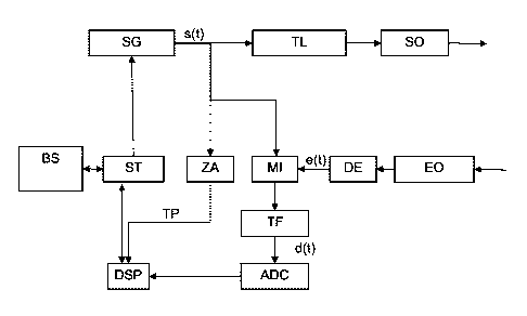
Fig. 1 shows the schematic diagram of a first working example according to the
invention, comprising a mixer MI into which the electrical signal s(t) of the
signal generator SG
and the echo signal e(t) of the detector DE are coupled. The signal s(t) of
the signal generator SG
is also used for superposing a frequency modulation on the radiation generated
by driver and
laser TL. This optical radiation in the visible or non-visible spectral range
is emitted via a
transmitting optical system SO and, after reflection by one or more targets or
objects, is received
again via a receiving optical system EO and a detector DE. In the homodyne
method, both the
signal s(t) of the signal generator SG and the signal of the beam generation
of driver and laser
TL, included in the received radiation, are used by the mixer MI. The result
of the mixer MI is
digitized via a low-pass filter TF and an analogue/digital converter AC and
fed to the digital
signal processor DSP for signal processing. In parallel with the mixer MI, the
total phase TP is
determined by a counter ZA and likewise fed to the digital signal processor
DSP. A control ST
controls the signal generator SG so that a deviation of the signal generation
from the ideal profile
9
CA 02583337 2014-03-21
can be compensated. Either the signal s(t) generated by the signal generator
SG can therefore be
varied by the control ST so that the actual emission has a linear frequency
profile or the error is
taken into account purely algorithmically in the evaluation. In addition,
corrections of the
deviation from ideal behaviour and computational consideration thereof can
also be combined.
The distance-measuring apparatus can be controlled via a user interface BS.
Fig. 2 schematically shows a second working example according to the
invention,
comprising a mixer MI with optically detected signal and a counter ZA for the
total phase TP. In
contrast to Fig. 1, the signal s(t) of the signal generator SG is not fed
directly to the mixer MI but
the radiation emitted by the driver and laser TL is passed via a beam splitter
SD to a second
detector DE2, the output of which is once again connected both to the mixer MI
and to a counter
ZA for determining the total phase TP. This arrangement therefore uses not
only the echo signal
e(t) but also a second optically detected signal s(t-to) which is fed via an
internal zone so that
influences of the driver/laser combination TL act equally on both signals of
the mixer MI.
A working example similar to Fig. 1 is shown in Fig. 3 as a schematic diagram
of a third
working example according to the invention, comprising two mixers, direct
electrical signal
incoupling and a quadrature receiver. The signal i(t) of the signal generator
SG is fed to a first
mixer MI1 and a second mixer MI2 with down-circuit low-pass filters TF and
analogue/digital
converters ADC, the signal of the second mixer MI2 being shifted in an 900
phase shifter. The
echo signal e(t) of the radiation registered by the detector DE is coupled
both into the first mixer
MI1 and into the second mixer MI2 so that a quadrature receiver results
overall.
Fig. 4 shows the schematic diagram of a fourth working example according to
the
invention which is similar to the second working example of Fig. 2 and
comprises two mixers,
optically detected signal s(t-to) and a quadrature receiver. This fourth
working example combines
the quadrature receiver of the third working example of Fig. 3 with the
optical detection of the
signal s(t-to) of the second working example of Fig. 2. In contrast to Fig. 1,
the signal s(t) of the
signal generator SG is not fed directly to the quadrature receiver, but the
radiation emitted by
driver and laser TL is passed via a beam splitter SD to a second detector DE2
which in turn is
connected to the quadrature receiver.
CA 02583337 2014-03-21
Fig. 5 schematically shows the generation of a mixed term by the sequence of
superposition UE and nonlinearity NL. This generation of a mixed term
represents a further
fundamental possibility which can be combined with any of the above working
examples. There
are advantages particularly in association with the second working example,
since a detector can
be omitted thereby. The replacement of a mixer is effected by superposition UE
of mixing signal
m(t) and echo signal e(t) before or at the detector DE with subsequent
nonlinearity NL and a low-
pass filter TF. A quadratic nonlinearity NL produces as a mixed term precisely
the desired
product, and the low-pass filtration TF suppresses the undesired turns. This
principle is used, for
example, in diode or FET mixers.
The following Fig. 6-11 show the effects of a deviation from the strictly
linear profile of
the chirp for a homodyne and a heterodyne example, from which errors in the
distance
measurement can result. Without modelling the chirp profile, either more
complicated apparatus
must be employed in order to meet the linearity requirements or measurements
containing errors
must be accepted.
Fig. 6-8 show numerical examples for the homodyne case. The simulations were
calculated by means of Matlab, the following values serving as basis:
f, = 10 MHz Sampling frequency
T = 1 ms Chirp duration
m = 9980 Number of sampling points
fo = 600 MHz Centre frequency
B = 100 MHz Chirp bandwidth
do = 0 Signal offset
For two equally strong targets at the distances 4.5 m and 45 m, Fig. 6 shows
the diagram
of the frequency profile (top) and of the mixed and sampled received signal
(bottom) for a perfect
linear chirp in the homodyne case.
Fig. 7 shows a disturbance of the ideal chirp in the homodyne case with an
additional
fourth-order term in equation (1). In order that starting and end frequency do
not change very
much, a slight adaptation of the quadratic term was also carried out. The
disturbance term in the
11
CA 02583337 2014-03-21
phase function is therefore
Acl)(t) = ¨6.0109s2 .t2 +1.114.1016S-4 .t4 (9)
Fig. 7 once again shows frequency profile (top) and mixed and sampled received
signal
(bottom).
Fig. 8 shows differences of emitted frequency and received signal between
disturbed and
ideal chirp in the homodyne case. Although the chirp frequency deviates only
by a maximum of
0.42% from the ideal value, the difference in the received signal is just as
large as the signal
itself The frequency difference (top) and the received signal difference
(bottom) are shown.
Fig. 9-11 show numerical examples for the heterodyne case. The simulations
were
likewise calculated by means of Matlab, the same values as in the homodyne
case serving as a
basis. The frequency fi of the harmonic mixing signal is fi = 500 MHz.
Fig. 9 shows the frequency profile (top) and the received signal (bottom) for
the linear
chirp in the heterodyne case. The same parameter values and the same target
distances as in the
above homodyne case are used.
Fig. 10 shows the effect of the disturbance according to equation (9) of the
ideal chirp in
the heterodyne case. Once again, frequency profile (top) and mixed and sampled
received signal
(bottom) are shown.
Fig. 11 shows the differences of emitted frequency and received signal between
disturbed
and ideal chirp in the heterodyne case. Although the chirp frequency deviates
only by a
maximum of 0.42% from the ideal value, the difference in the received signal
is once again just
as large as the signal itself
It is of course self-evident to the person skilled in the art that the various
arrangements of
components or principles can be combined with one another in an alternative or
supplementary
manner. The working examples of the apparatuses can ¨ as already mentioned ¨
also be designed
in heterodyne or homodyne construction, with mixers of different design, such
as, for example,
Gilbert cells or sampling mixers, or with replacement of one or more mixers by
the sequence of
superposition and nonlinearity.
12