Note : Les descriptions sont présentées dans la langue officielle dans laquelle elles ont été soumises.
CA 02733032 2011-02-28
Method and Apparatus for Improved Navigation of a Moving Platform
FIELD OF THE INVENTION
The present invention relates to positioning and navigation systems adapted
for use in environments with good, degraded, or denied satellite-based
navigation
signals.
BACKGROUND OF THE INVENTION
The positioning of a moving platform, such as, wheel-based
platforms/vehicles or individuals, is commonly achieved using known reference-
based systems, such as the Global Navigation Satellite Systems (GNSS). The
GNSS
comprises a group of satellites that transmit encoded signals and receivers on
the
ground, by means of trilateration techniques, can calculate their position
using the
travel time of the satellites' signals and information about the satellites'
current
location.
Currently, the most popular form of GNSS for obtaining absolute position
measurements is the global positioning system (GPS), which is capable of
providing
accurate position and velocity information provided that there is sufficient
satellite
coverage. However, where the satellite signal becomes disrupted or blocked
such as,
for example, in urban settings, tunnels and other GNSS-degraded or GNSS-denied
environments, a degradation or interruption or "gap" in the GPS positioning
information can result.
In order to achieve more accurate, consistent and uninterrupted positioning
information, GNSS information may be augmented with additional positioning
information obtained from complementary positioning systems. Such systems may
be
self-contained and/or "non-reference based" systems within the platform, and
thus
need not depend upon external sources of information that can become
interrupted or
blocked.
One such "non-reference based" or relative positioning system is the inertial
navigation system (INS). Inertial sensors are self-contained sensors within
the
platform that use gyroscopes to measure the platform's rate of rotation/angle,
and
accelerometers to measure the platform's specific force (from which
acceleration is
CA 02733032 2011-02-28
obtained). Using initial estimates of position, velocity and orientation
angles of the
moving platform as a starting point, the INS readings can subsequently be
integrated
over time and used to determine the current position, velocity and orientation
angles
of the platform. Typically, measurements are integrated once for gyroscopes to
yield
orientation angles and twice for accelerometers to yield position of the
platform
incorporating the orientation angles. Thus, the measurements of gyroscopes
will
undergo a triple integration operation during the process of yielding
position. Inertial
sensors alone, however, are unsuitable for accurate positioning because the
required
integration operations of data results in positioning solutions that drift
with time,
thereby leading to an unbounded accumulation of errors.
Another known complementary "non-reference based" system is a system for
measuring speed/velocity information such as, for example, odometric
information
from a odometer within the platform. Odometric data can be extracted using
sensors
that measure the rotation of the wheel axes and/or steer axes of the platform.
Wheel
rotation information can then be translated into linear displacement, thereby
providing
wheel and platform speeds, resulting in an inexpensive means of obtaining
speed with
relatively high sampling rates. Where initial position and orientation
estimates are
available, the odometric data are integrated thereto in the form of
incremental motion
information over time.
Odometry has short-term accuracy, however, odometric data can contain
errors such as those that may arise from wheel slippage. If odometry is to be
used
alone to obtain a positioning solution (i.e. using it to get both
translational speed of
the platform as well as rotational motion), the integration of motion
information
including errors such as wheel slippage will result in the small errors
increasing
without bound over time because of integration operations. For instance, it is
known
that orientation errors can create large positional errors that increase with
the distance
traveled by the platform.
Given that each positioning technique described above (INS/GNSS/Speed
Information) may suffer loss of information or errors in data, common practice
involves integrating the information/data obtained from the GNSS with that of
the
complementary system(s). For instance, to achieve a better positioning
solution, INS
and GPS data may be integrated because they have complementary
characteristics.
2
CA 02733032 2011-02-28
INS readings are accurate in the short-term, but their errors increase without
bounds
in the long-term due to inherent sensor errors. GNSS readings are not as
accurate as
INS in the short-term, but GNSS accuracy does not decrease with time, thereby
providing long-term accuracy. Also, GNSS may suffer from outages due to signal
blockage, multipath effects, interference or jamming, while INS is immune to
these
effects.
Although available, integrated INS/GNSS is not often used commercially for
low cost applications because of the relatively high cost of navigational or
tactical
grades of inertial measurement units (IMUs) needed to obtain reliable
independent
positioning and navigation during GNSS outages. Low cost, small, lightweight
and
low power consumption Micro-Electro-Mechanical Systems (MEMS)-based inertial
sensors may be used together with low cost GNSS receivers, but the performance
of
the navigation system will degrade very quickly in contrast to the higher
grade IMUs
in areas with little or no GNSS signal availability due to time-dependent
accumulation
of errors from the INS.
Speed information from the odometric readings, or from any other source,
may be used to enhance the performance of the MEMS-based integrated INS/GNSS
solution by providing velocity updates, however, current INS/Odometry/GNSS
systems continue to be plagued with the unbounded growth of errors over time
during
GNSS outages.
One reason for the continued problems is that commercially available
navigation systems using INS/GNSS integration or INS/Odometry/GNSS integration
rely on the use of traditional Kalman Filter (KF)-based techniques for sensor
fusion
and state estimation. The KF is an estimation tool that provides a sequential
recursive
algorithm for the estimation of the state of a system when the system model is
linear.
As is known, the KF estimates the system state at some time point and then
obtains observation "updates" in the form of noisy measurements. As such, the
equations for the KF fall into two groups:
= Time update or "prediction" equations: used to project forward in time
the current state and error covariance estimates to obtain an a priori
estimate for the next step, or
3
CA 02733032 2011-02-28
= Measurement update or "correction" equations: used to incorporate a
new measurement into the a priori estimate to obtain an improved
posteriori estimate.
While the commonly used Linearalized KF (LKF) and Extended KF (EKF)
can provide adequate solutions when higher grade IMUs are utilized by
linearizing the
originally nonlinear models, the KF generally suffers from a number of major
drawbacks that become influential when using low cost MEMS-based inertial
sensors,
as outlined below.
The INS/GNSS integration problem at hand has nonlinear models. Thus, in
order to utilize the linear KF estimation techniques in this type of problem,
the
nonlinear INS/GNSS model has to be linearized around a nominal trajectory.
This
linearization means that the original (nonlinear) problem be transformed into
an
approximated problem that may be solved optimally, rather than approximating
the
solution to the correct problem. The accuracy of the resulting solution can
thus be
reduced due to the impact of neglected nonlinear and higher order terms. These
neglected higher order terms are more influential and cause error growth in
the
positioning solution, in degraded and GNSS-denied environments, particularly
when
low cost MEMS-based IMUs are used.
Further, the KF requires an accurate stochastic model of each of the inertial
sensor errors, which can be difficult to obtain, particularly where low cost
MEMS-
based sensors are used because they suffer from complex stochastic error
characteristics. The KF is restricted to use only linear low-order (low memory
length)
models for these sensors' stochastic errors such as, for example, random walk,
Gauss-
Markov models, first order Auto-Regressive models or second order Auto-
Regressive
models. The dependence of the KF on these inadequate models is also a drawback
of
the KF when using low cost MEMS-based inertial sensors.
As a result of these shortcomings, the KF can suffer from significant drift or
divergence during long periods of GNSS signal outages, especially where low
cost
sensors are used. During these periods, the KF operates in prediction mode
where
errors in previous predictions, which are due to the stochastic drifts of the
inertial
sensor readings not well compensated by linear low memory length sensors'
error
models and inadequate linearized models, are propagated to the current
estimate and
4
CA 02733032 2011-02-28
summed with new errors to create an even larger error. This propagation of
errors
causes the solution to drift more with time, which in turn causes the
linearization
effect to worsen because of the drifting solution used as the nominal
trajectory for
linearization (in both LKF and EKF cases). Thus, the KF techniques suffer from
divergence during outages due to approximations during the linearization
process and
system mis-modeling, which are influential when using MEMS-based sensors.
In addition, the traditional INS typically relies on a full inertial
measurement
unit (IMU) having three orthogonal accelerometers and three orthogonal
gyroscopes.
This full IMU setting has several sources of error, which, in the case of low-
cost
MEMS-based IMUs, will cause severe effects on the positioning performance. The
residual uncompensated sensor errors, even after KF compensation, can cause
position error composed of three additive quantities: (i) proportional to the
cube of
GNSS outage duration and the uncompensated horizontal gyroscope biases; (ii)
proportional to the square of GNSS outage duration and the three
accelerometers
uncompensated biases, and (iii) proportional to the square of GNSS outage
duration,
the horizontal speed, and the vertical gyroscope uncompensated bias.
Another traditional solution, known as Dead reckoning, which can be used to
provide a two dimensional (2D) positioning solution for land vehicles using a
single
axis gyroscope vertically aligned with the vehicle and the speed readings from
an
odometer. Dead reckoning relies on an assumption that vehicles will primarily
move
on the horizontal plane. However, this solution is also plagued with certain
drawbacks, namely: (i) it is a 2D solution that does not estimate the altitude
nor the
vertical component of velocity; and (ii) assuming that the vehicle is moving
in the
horizontal plane, it disregards the tilt angles of the vehicles and
subsequently the off-
plane motion which causes two main issues: (a) the assumption that the
gyroscope
vertically aligned to the vehicle also has its axis in the pure vertical (i.e.
normal to the
East-North plane), which is a problem because its axis is actually tilted,
will affect the
accuracy of the azimuth calculation, and (b) the assumption that the vehicle's
traveled
path is horizontal, which is a problem because the vehicle and its path are
actually
tilted, will cause an error in the horizontal position estimation.
The foregoing drawbacks of the KF have resulted in increased investigation
into alternative methods of INS/GNSS integration models, such as, for example,
5
CA 02733032 2011-02-28
nonlinear artificial intelligence techniques. However, there is a need for
enhancing the
performance of low-end systems relying on low cost MEMS-based INS/GNSS
sensors and for mitigating the effect of all sources of errors to provide a
more
adequate navigation solution. Further, there is also a need for more advanced
modeling techniques that are capable of modeling the stochastic sensor errors
instead
of the linear low memory length models currently used.
SUMMARY
A navigation module for providing an INS/GNSS navigation solution for a
moving platform is provided. A method of using the navigation module to
determine
an INS/GNSS navigation solution is also provided.
The module comprises a receiver for receiving absolute navigational
information about the moving platform from an external source (e.g., such as a
satellite), and producing an output of navigational information indicative
thereof.
The module further comprises means for obtaining speed or velocity
information and producing an output of information indicative thereof.
The module further comprises an assembly of self-contained sensors capable
of obtaining readings (e.g., such as relative or non-reference based
navigational
information) and producing an output indicative thereof for generating
navigational
information. The sensor assembly may comprise accelerometers, gyroscopes,
magnetometers, barometers, and any other self-contained sensing means that are
capable of generating navigational information. More specifically, where the
means
for generating speed or velocity information (e.g., such as an odometer), is
capable of
providing uninterrupted information to the module, the sensor assembly may
comprise at least two accelerometers and one gyroscope. Alternatively, where
the
means for generating speed or velocity information is subject to interruption
(e.g. such
as platforms having transceivers that enables them to get their own Doppler-
derived
velocities), the sensor assembly may comprise three accelerometers and three
gyroscopes.
Finally, the module further comprises at least one processor, coupled to
receive the output information from the receiver, sensor assembly and means
for
obtaining speed or velocity information, and operative to integrate the output
6
CA 02733032 2011-02-28
information to produce a navigation solution. The at least one processor may
operate
to provide a navigation solution by using the speed or velocity information to
decouple the actual motion of the platform from the readings of the sensor
assembly.
The processor may be programmed to utilize a filtering technique, such as a
non-
linear filtering technique (e.g., a Mixture Particle Filter), and the
integration of the
information from different sources may be done in either loosely or tightly
coupled
integration schemes. The filtering algorithm may utilize a system model and a
measurement model, wherein the system and measurement model used by the
algorithm may depend upon whether or not the speed or velocity information
available to the module can be interrupted. The system and measurement models
utilized by the present navigation module provides new combinations of sensor
assembly and speed or velocity information and enhanced navigation solutions
relating to a moving platform, even in circumstances of degraded or denied
GNSS
information.
A method for determining an improved navigation solution is further provided
comprising the steps of:
a) receiving absolute navigational information from an external source and
producing output readings indicative thereof;
b) obtaining readings relating to navigational information at self-contained
sensors within the module and producing an output indicative thereof;
c) obtaining speed or velocity information and producing output readings
indicative thereof; and
d) providing at least one processor for processing and filtering the
navigational
information and speed or velocity information to produce a navigation solution
relating to the module, wherein the at least one processor is capable of
utilizing the
speed or velocity readings to decouple the actual motion of the platform from
the
sensor information.
Where, the navigation module comprises a non linear state estimation or
filtering technique, such as, for example, Mixture Particle Filter for
performing
INS/GNSS integration, the module may be optionally enhanced to provide
advanced
modeling of inertial sensors stochastic drift together with the derivation of
measurement updates for such drift.
7
CA 02733032 2011-02-28
The module may be optionally programmed to detect and assess the quality of
GNSS information received by the module and, where degraded, automatically
discard or discount the information.
The module may be optionally enhanced to automatically switch between a
loosely coupled integration scheme and a tightly coupled integration scheme.
The module may be optionally enhanced to automatically assess
measurements from each external source, or GNSS satellite visible to the
module in
case of a tightly coupled integration scheme, and detect degraded
measurements.
The module may be optionally enhanced to calculate misalignment between
the sensor assembly of the module and the platform.
The module may be optionally enhanced to perform a backward or post-
mission process to calculate a solution subsequent to the forward navigation
solution,
and to blend the two solutions to provide an enhanced backward smoothed
solution.
The module may be optionally enhanced to perform one or more of any of the
foregoing options.
DESCRIPTION OF THE DRAWINGS
Figures 1: A diagram demonstrating the present navigation module as defined
herein.
Figure 2A: A flow chart diagram demonstrating the present navigation module
of Figure 1(dashed lines and arrows depict optional processing).
Figure 2B: A flow chart diagram demonstrating the optional post-mission
embodiment of the present navigation module defined herein.
Figure 3: Road Test Trajectory in Montreal, Quebec, Canada. Circles indicate
the locations of GPS outages.
Figure 4: Performance during GPS outage #3 of Figure 3.
Figure 5: Performance during GPS outage #4 of Figure 3.
Figure 6: Performance during GPS outage #9 of Figure 3.
Figure 7: Forward speed, azimuth, altitude, and pitch during GPS outage #3 in
Figures 3 and 4.
Figure 8: Forward speed, azimuth, altitude, and pitch during GPS outage #4 in
Figures 3 and 5.
8
CA 02733032 2011-02-28
Figure 9: Forward speed, azimuth, altitude, and pitch during GPS outage #9 in
Figures 3 and 6.
Figure 10: Road Test Trajectory between Kingston and Napanee, Ontario,
Canada. Circles indicate the locations of GPS outages.
Figure 11: Performance during GPS outage #3 as shown in Figure 10.
Figure 12: Performance during GPS outage #5 as shown in Figure 10.
Figure 13: Performance during GPS outage #8 as shown in Figure 10.
Figure 14: Forward speed and azimuth from NovAtel reference during GPS
outage #3 of Figures 10 and 11.
Figure 15: Forward speed and azimuth from NovAtel reference during GPS
outage #5 of Figures 10 and 12.
Figure 16: Forward speed and azimuth from NovAtel reference during GPS
outage #8 of Figures 10 and 13.
Figure 17: The autocorrelation of gyroscope reading of the second stationary
dataset.
Figure 18: The autocorrelation of gyroscope reading of the second stationary
dataset after removing the initial bias offset.
Figure 19: The gyroscope reading of the second stationary dataset after
removing the initial bias offset versus the PCI prediction of the drift.
Figure 20: The autocorrelation of gyroscope reading of the second stationary
dataset after removing the initial bias offset and the PCI predicted drift.
Figure 21: The gyroscope reading of the second stationary dataset after
removing the initial bias offset versus the AR prediction of the drift.
Figure 22: The autocorrelation of gyroscope reading of the second stationary
dataset after removing the initial bias offset and the AR predicted drift.
Figure 23: Road Test Trajectory from Montreal to Kingston. Circles indicate
the locations of GPS outages.
Figure 24: Performance during GPS outage #8 shown in Figure 23.
Figure 25: Forward speed and azimuth from Novatel reference during GPS
outage #8 shown in Figure 23 and 24.
Figure 26: Performance during GPS outage #9 shown in Figure 23.
9
CA 02733032 2011-02-28
Figure 27: Forward speed and azimuth from Novatel reference during GPS
outage #9 shown in Figure 23 and 26.
Figure 28: Performance during GPS outage #10 shown in Figure 23.
Figure 29: Forward speed and azimuth from Novatel reference during GPS
outage #10 shown in Figure 23 and 28.
Figure 30: Road Test Trajectory in Toronto, Coming from North to South into
downtown then leaving from the South-East.
Figure 31: Zoom-in on first portion of degraded GPS performance in Toronto
trajectory of Figure 30.
Figure 32: Zoom-in on second portion of degraded GPS performance in
Toronto trajectory of Figure 30.
Figure 33: Zoom-in on third and hardest portion of degraded GPS
performance in Toronto trajectory of Figure 30.
Figure 34: Zoom-in on a section with complete blockage under the Gardiner
Expressway in Toronto trajectory of Figure 30.
Figure 35: Comparison between Mixture PF/AR120 and KF/GM both with
gyroscope drift update and automatic detection of GPS degraded performance of
Figure 30.
Figure 36: Road Test Trajectory around Kingston, Ontario, Canada area.
Circles indicate the locations of GPS outages.
Figure 37: Number of satellites visible to the NovAtel OEM4 receiver during
the Kingston Trajectory.
Figure 38: Average RMS position error over the ten 60-second outages in
Kingston trajectory with different numbers of satellites visible (3, 2, 1, and
0).
Figure 39: Average maximum position error over the ten 60-second outages in
Kingston trajectory with different numbers of satellites visible (3, 2, 1, and
0).
Figure 40: Performance during GPS outage #5 as shown in Figure 36.
Figure 41: Performance towards the end of GPS outage #5 as shown in Figure
36.
Figure 42: Forward speed and azimuth from Novatel reference during GPS
outage #5 as shown in Figure 36 and 40.
Figure 43: Performance during GPS outage #7 as shown in Figure 36.
CA 02733032 2011-02-28
Figure 44: Performance towards the end of GPS outage #7 as shown in Figure
43.
Figure 45: Forward speed and azimuth from Novatel reference during GPS
outage #7 as shown in Figure 36 and 43.
Figure 46: Road Test Trajectory in Toronto that starts and ends in the North,
having the downtown area in the south of the trajectory.
Figure 47: Zoom in on the downtown portion of the Toronto trajectory shown
in Figure 46.
Figure 48: Number of GNSS satellites (GPS+GLONASS) visible to the
NovAtel OEMV-1G receiver during the Toronto trajectory shown in Figure46.
Figure 49: Number of GPS-only satellites visible to the NovAtel OEMV-1G
receiver during the Toronto trajectory shown in Figure 46.
Figure 50: Zoom in on the downtown portion of the Toronto trajectory shown
in Figure 46 showing the degraded GPS performance and the performance of the
proposed navigation solution.
Figure 51: More detailed view on the downtown portion of the Toronto
trajectory shown in Figure 46 showing the degraded GPS performance and the
performance of the proposed navigation solution.
Figure 52: Road Test Trajectory in Houston, Texas.
Figure 53: One outage in a road covered by dense trees during the Houston
trajectory of Figure 52.
Figure 54: Different outages when moving at slow speed in the vicinity of a
building with some roof top canopies during the Houston trajectory of Figure
52.
Figure 55: An outage when passing under an overpass during the Houston
trajectory of Figure 52.
Figure 56: Road Test Trajectory in Downtown Toronto, a slightly zoomed in
portion of trajectory shown in Figure 30.
Figure 57: Comparisons of the forward and backward proposed solutions, with
GPS, and reference in a portion of downtown Toronto shown in Figure 52 with
severe
GPS degradations and blockages.
11
CA 02733032 2011-02-28
Figure 58: Comparisons of the forward and backward solutions, with GPS,
and reference in another portion of downtown Toronto shown in Figure 52 with
severe GPS degradations and blockages.
Figure 59: Comparisons of the forward and backward solutions, with GPS,
and reference in the portion of the downtown Toronto shown in Figure 52 with
the
worst GPS degradations and blockages.
Figure 60: Comparisons of the forward and backward solutions, with GPS,
and reference in a complete blockage under Gardiner Expressway in Toronto
trajectory shown in Figure 52.
Figure 61: Comparisons of the forward and backward solutions, with GPS,
and reference in another complete blockage under Gardiner Expressway in
Toronto
trajectory shown in Figure 52.
Table 1: RMS horizontal position error during GPS outages for Montreal
trajectory shown in Figure 3.
Table 2: Maximum horizontal position error during GPS outages for Montreal
trajectory.
Table 3: RMS altitude error during GPS outages for the Montreal trajectory.
Table 4: Maximum altitude error during GPS outages for Montreal trajectory.
Table 5: RMS horizontal position error during 120 sec. GPS outages for
Kingston-Napanee trajectory.
Table 6: Maximum horizontal position error during 120 sec. GPS outages for
Kingston-Napanee trajectory.
Table 7: RMS altitude error during 120 sec. GPS outages for Kingston-
Napanee trajectory.
Table 8: Maximum altitude error during 120 sec. GPS outages for Kingston-
Napanee trajectory.
Table 9: RMS horizontal position error during 60 sec. GPS outages for
Montreal-Kingston trajectory.
Table 10: Maximum horizontal position error during 60 sec. GPS outages for
Montreal-Kingston trajectory.
Table 11: RMS horizontal position error during 180 sec. GPS outages for
Montreal-Kingston trajectory.
12
CA 02733032 2011-02-28
Table 12: Maximum horizontal position error during 180 sec. GPS outages for
Montreal-Kingston trajectory.
Table 13: Maximum position error during the 10 simulated outages for
different numbers of visible satellites.
Table 14: RMS and maximum position error for the natural GPS degradation
or blockage periods whose duration exceeds 100 sec in the Toronto trajectory
shown
in Figure 46.
Table 15: Crossbow 300CC IMU specifications.
Table 16: Analog Devices ADIS16405 IMU Specifications.
Table 17: Honeywell HG1700 IMU Specifications.
Table 18: Benchmarking results for different GNSS outages durations with
over 100. randomly simulated outages for each duration.
DESCRIPTION OF THE PREFERRED EMBODIMENT
An improved navigation module and method for providing an INS/GNSS
navigation solution for a moving platform is provided. More specifically, the
present
navigation module and method for providing a navigation solution may be used
as a
means of overcoming inadequacies of (i) traditional full IMU/GNSS integration,
traditional full IMU/Odometry/GNSS integration, and traditional 2D dead
reckoning/GNSS integration; (ii) commonly used linear state estimation
techniques
where low cost inertial sensors are used, particularly in circumstances where
positional information from the GNSS is degraded or denied, such as in urban
canyons, tunnels and other such environments. Despite such degradation or
denial of
GNSS information, the present navigation module and method of producing
navigational information may provide uninterrupted navigational information
about
the moving platform by augmenting the INS/GNSS information with additional
complementary sources of information. The type of complementary information
used,
and how such information is used, may depend upon the assembly of the
navigation
module and the use thereof.
13
CA 02733032 2011-02-28
Navigation Module
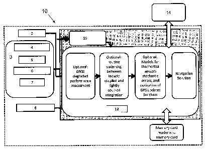
The present navigation module 10 (Figure 1) may comprise means for receiving
"absolute" or "reference-based" navigation information 2 about a moving
platform
from external sources, such as satellites, whereby the receiving means is
capable of
producing an output indicative of the navigation information. For example, the
receiver means may be a GNSS receiver capable of receiving navigational
information from GNSS satellites and converting the information into position,
and
velocity information about the moving platform. The GNSS receiver may also
provide
navigation information in the form of raw measurements such as pseudoranges
and
Doppler shifts.
In one embodiment, the GNSS receiver may be a Global Positioning System
(GPS) receiver, such as a uBlox LEA-5T receiver module. It is to be understood
that
any number of receiver means may be used including, for example and without
limitation, a NovAtel OEM 4 dual frequency GPS receiver, a NovAtel OEMV-1G
single frequency GPS receiver, or a Trimble Lassen SQ GPS receiver, which is a
single frequency low-end receiver with access to GPS only.
The present navigation module may also comprise self-contained sensor
means 3, in the form of a sensor assembly, capable of obtaining or generating
"relative" or "non-reference based" readings relating to navigational
information
about the moving platform, and producing an output indicative thereof For
example,
the sensor assembly may be made up of accelerometers 4, for measuring
accelerations, and gyroscopes 5, for measuring turning rates of the moving
platform.
Optionally, the sensor assembly may have other self-contained sensors such as,
without limitation, magnetometers 6, for measuring magnetic field strength for
establishing heading, barometers 7, for measuring pressure to establish
altitude, or any
other sources of "relative" navigational information.
In one embodiment, the sensor assembly may comprise orthogonal Micro-
Electro-Mechanical Systems (MEMS) accelerometers, and MEMS gyroscopes, such
as, for example, those obtained in one inertial measurement unit package from
Analog
Devices Inc. (ADI) Model No. ADIS16405, and may or may not include orthogonal
magnetometers available in the same package or in another package such as, for
14
CA 02733032 2014-10-02
example model HMC5883L from Honeywell, and barometers such as, for example,
(model MS5803) from Measurement Specialties.
More specifically, if circumstances arise where means of speed or velocity
reading information is available and uninterrupted, one embodiment of the
present
navigation module may comprise a sensor assembly having a reduced number of
inertial sensors with at least two accelerometers in the longitudinal and
lateral
directions of the moving platform, and one vertical gyroscope for monitoring
heading
rate of the platform. In one embodiment, the sensor assembly comprises two
accelerometers (in the longitudinal and lateral directions) and one gyroscope.
Optionally, other self-contained sources of navigational information such as,
for
example, magnetometers and/or barometers and/or a third vertical accelerometer
may
be added.
In circumstances where means of speed reading or velocity information is
available, but interrupted, another embodiment of the present navigation
module may
comprise a traditional sensor assembly having three accelerometers in the
longitudinal, lateral and vertical directions of the moving platform, and
between one
and three vertical gyroscopes (two for measuring roll and pitch, and a
vertical
gyroscope for measuring heading). Optionally, other self-contained sources of
navigational information such as, for example, magnetometers and/or barometers
may
be added.
Third, the present navigation module may comprise means for or a source for
obtaining speed and/or velocity information 8 of the moving platform, wherein
said
source is capable of further generating an output or "reading" indicative
thereof
While it is understood that such source can be either speed and/or velocity
information, said source shall only be referenced herein as a source of speed
information. In one embodiment, the source for generating speed information
may
comprise an odometer, a wheel-encoder, shaft or motor encoder of any wheel-
based
or track-based platform, or to any other source of speed and/or velocity
readings (for
example, those derived from Doppler shifts of any type of transceiver). In a
preferred
embodiment, the source for generating speed is the built-in odometer of the
platform.
The source of obtaining speed information, such as the odometer, may be
connected
to the Controller Area Network (CAN) bus or the On Board Diagnostics version
II
CA 02733032 2014-10-02
(OBD-II) of the platform. It should be understood that the means or source for
generating speed/velocity information about the moving platform may be
connected
to the navigation module via wired or wireless connection.
Finally, the present navigation module 10 may comprise at least one processor
12 or microcontroller coupled to the module for receiving and processing the
foregoing absolute navigation 2, sensor assembly 3 and speed information 8,
and
determining a navigation solution output using the speed information to
decouple the
actual motion of the platform from the sensor assembly information. In both
circumstances of GNSS availability and interruption, the decoupling of the
information may occur by way of mathematical system and measurement models
that
the processor is programmed to use (Figure 2A), however the models differ in
each
case, as discussed in detail below.
The navigation solution determined by the present navigation module 10 may
be communicated to a display or user interface 14. It is contemplated that the
display
14 be part of the module 10, or separate therefrom (e.g., connected wired or
wirelessly
thereto). The navigation solution determined in real-time by the present
navigation
module 10 may further be stored or saved to a memory device/card 16
operatively
connected to the module 10.
In one embodiment, a single processor such as, for example, ARM Cortex R4
or an ARM Cortex A8 may be used to integrate and process the signal
information. In
another embodiment, the signal information may initially be captured and
synchronized by a first processor such as, for example, an ST Micro (STM32)
family
or other known basic microcontroller, before being subsequently transferred to
a
second processor such as, for example, ARM Cortex R4 or ARM Cortex A8.
The processor may be programmed to use known state estimation techniques
to provide the navigation solution. In one embodiment, the state estimation
technique
may be a non-linear technique. In a preferred embodiment, the processor may be
programmed to use the non-linear Particle Filter (PF) or the Mixture PF. In
another
embodiment, the processor may be programmed to use a linear state estimation
technique, thereby necessitating linearization of the information.
It is an object of the present navigation module 10 to produce three
dimensional
(3D) position, velocity and orientation information for any moving platform
that is, for
example, wheel-based, track-based or has a source of speed or
16
CA 02733032 2011-02-28
velocity readings (whether interrupted or not), particularly for circumstances
where
positional information from the GNSS is degraded or denied. It is a further
object that
the integrated navigation solution may be operable in land-based wheeled
platforms
such as automobiles, machinery with wheels, mobile robots and wheelchairs, or
with
any non-wheeled system provided that they have means of measuring speed or
velocity (for example Doppler-derived velocity).
It is known that there are three main types of INS/GNSS integration that have
been proposed to attain maximum advantage depending upon the type of use and
choice of simplicity versus robustness. This leads to three main integration
architectures:
1. Loosely coupled
2. Tightly coupled
3. Ultra-tightly coupled (or deeply coupled).
The first type of integration, which is called loosely coupled, uses an
estimation
technique to integrate inertial sensors data with the position and velocity
output of a
GNSS receiver. The distinguishing feature of this configuration is a separate
filter for
the GNSS. This integration is an example of cascaded integration because of
the two
filters (GNSS filter and integration filter) used in sequence.
The second type, which is called tightly coupled, uses an estimation technique
to integrate inertial sensors readings with raw GNSS data (i.e. pseudoranges
that can
be generated from code or carrier phase or a combination of both, and
pseudorange
rates that can be calculated from Doppler shifts) to get the vehicle position,
velocity,
and orientation. In this solution, there is no separate filter for GNSS, but
there is a
single common master filter that performs the integration.
For the loosely coupled integration scheme, at least four satellites are
needed to
provide acceptable GNSS position and velocity input to the integration
technique. The
advantage of the tightly coupled approach is that less than four satellites
can be used
as this integration can provide a GNSS update even if fewer than four
satellites are
visible, which is typical of a real life trajectory in urban environments as
well as thick
forest canopies and steep hills. Another advantage of tightly coupled
integration is
that satellites with poor GNSS measurements can be detected and rejected from
being
used in the integrated solution.
17
CA 02733032 2011-02-28
For the third type of integration, which is ultra-tight integration, there are
two
major differences between this architecture and those discussed above.
Firstly, there is
a basic difference in the architecture of the GNSS receiver compared to those
used in
loose and tight integration. Secondly, the information from INS is used as an
integral
part of the GNSS receiver, thus, INS and GNSS are no longer independent
navigators,
and the GNSS receiver itself accepts feedback. It should be understood that
the
present navigation solution may be utilized in any of the foregoing types of
integration.
In one embodiment, the present navigation module 10 may operate to
determine a three dimensional (3D) navigation solution by calculating 3D
position,
velocity and attitude of a moving platform, wherein the navigation module
comprises
absolute navigational information from a GNSS receiver, the self-contained
sensors
which are MEMS-based reduced inertial sensor systems comprising two orthogonal
accelerometers and one single-axis gyroscope vertically aligned to the
platform,
speed/velocity information from the odometer of the moving platform, and a
processor programmed to integrate the information using Mixture PF in a
loosely
coupled architecture, having a system and measurement model, wherein the
system
model is capable of utilizing the speed information to decouple the actual
motion of
the platform from the readings of the accelerometers (see Example 1).
In another embodiment, the present navigation module may operate to
determine a 3D navigation solution by calculating position, velocity and
attitude of a
moving platform, wherein the module comprises a full (three orthogonal
accelerometers and three orthogonal gyroscopes) MEMS-based INS/GNSS
integration using Mixture PF in a loosely coupled architecture while using the
decoupling idea to provide extra measurement updates during GNSS availability
and/or during GNSS outages (see Example 2).
In another embodiment, the present navigation module may optionally be
programmed to utilize an enhanced loosely-coupled Mixture PF INS/GNSS
integration, wherein the integration further comprises the advanced modeling
of
inertial sensors stochastic drift together with the derivation of updates for
such drift
from GNSS, where appropriate (see Example 3).
18
CA 02733032 2011-02-28
In another embodiment, the present navigation module may also optionally be
programmed to automatically detect and assess the quality of GNSS information,
and
further provide a means of discarding or discounting degraded information (see
Example 4).
In another embodiment, the present navigation module may optionally be
programmed to utilize a Mixture PF for tightly-coupled INS/GNSS integration
(see
Example 5 ¨ Kingston Trajectory). In another embodiment, the navigation module
may optionally be further programmed to elect information between a loosely
coupled
and a tightly coupled integration scheme (see Example 5 ¨ Toronto Trajectory).
Moreover, where tightly coupled architecture is elected, the GNSS information
from
each available satellite may be assessed independently and either discarded
(where
degraded) or utilized as a measurement update (see Example 5 ¨ Toronto
Trajectory).
In another embodiment, the present navigation module may optionally be
programmed to operate an alignment procedure, which may be performed to
calculate
the orientation of the housing or frame of the sensor assembly within the
frame of the
moving platform, such as, for example the technique described in Example 7.
In another embodiment, the present navigation module may optionally be
programmed to detect stopping periods, known as zero velocity update (zupt)
periods,
either from the speed or velocity readings, from the inertial sensors
readings, or from
a combination of both. The detected stopping periods may be used to perform
explicit
zupt updates if the speed or velocity readings are interrupted. It is to be
noted that in
the case where the speed or velocity readings are uninterrupted, no explicit
zupt
update is needed because it is always implicitly performed. The detected
stopping
periods may be also used to automatically recalculate the biases of the
inertial sensors.
In another embodiment, the present navigation module may optionally be
programmed to determine a low-cost backward smoothed positioning solution for
a
moving platform with speed or velocity readings (whether interrupted or not),
such a
positioning solution might be used, for example, by mapping systems (see
Figure 3
and Example 6). In one embodiment, the foregoing navigation module utilizing
low-
cost MEMS inertial sensors, the platform's odometer and GNSS along with a
nonlinear filtering technique, may be further enhanced by exploiting the fact
that
19
CA 02733032 2011-02-28
mapping problem accepts post-processing and that nonlinear backward smoothing
may be achieved (see Figure 2B).
It is contemplated that the present system and/or measurement models, relying
on the fact that the motion of the moving platform detected from the speed or
velocity
readings (whether uninterrupted or interrupted) is decoupled from the sensors
assembly readings, can be used with any type of state estimation technique or
filtering
technique, for e.g., linear or non-linear techniques alone or in combination.
If the
technique is nonlinear, the nonlinear system and measurement models are
utilized as
defined herein. If the state estimation technique is linear, for example a
Kalman filter
(KF)-based technique, the present nonlinear system and measurement models will
be
linearized to be used as the system and measurement model inside the KF. In
the latter
circumstance, the present nonlinear system model will be used without the
process
noise terms in what is called "mechanization", which provides the nominal
solution
around which the linearization is performed. This mechanization can be an
unaided
mechanization in case of open loop systems or an aided mechanization that
receives
feedback from the estimated solution in the case of closed loop systems.
It is contemplated that the optional modules presented above can be used with
other sensors combinations (i.e. different system and measurement models) not
just
those used in the present navigation module relying on the fact that the
motion of the
moving platform detected from the speed or velocity readings (whether
uninterrupted
or interrupted) is decoupled from the sensors assembly readings. The optional
modules are the advanced modeling of inertial sensors errors, the derivation
of
possible measurements updates for them from GNSS when appropriate, the
automatic
assessment of GNSS solution quality and detecting degraded performance, the
automatic switching between loosely and tightly coupled integration schemes,
the
assessment of each visible GNSS satellite when in tightly coupled mode, the
alignment detection module, the automatic zupt detection with its possible
updates
and inertial sensors bias recalculations, and finally the backward smoothing
technique. For example, the optional modules can be used with navigation
solutions
relying on a 2D dead reckoning or a traditional full IMU
CA 02733032 2011-02-28
It is contemplated that the optional modules presented above can be used with
navigation solutions relying on either linear or nonlinear state estimation
techniques
or filtering techniques.
It is further contemplated that the present navigation module comprising a new
combination of speed readings and the inertial sensors can also be used
(whether with
linear or nonlinear filtering techniques) together with modeling (whether with
linear
or nonlinear, short memory length or long memory length) and/or automatic
calibration for the errors in speed or velocity readings. It is also
contemplated that
modeling (whether with linear or nonlinear, short memory length or long memory
length) and/or calibration for the other errors of inertial sensors (not just
the stochastic
drift) can be used. It is also contemplated that modeling (whether with linear
or
nonlinear, short memory length or long memory length) and/or calibration for
the
other sensors in the sensor assembly (such as, for example the barometer and
magnetometer) can be used.
It is further contemplated that the other sensors in the sensor assembly such
as,
for example, the barometer (e.g. with the altitude derived from it) and
magnetometer
(e.g. with the heading derived from it) can be used in one or more of
different ways
such as: (i) as control input to the system model of the filter (whether with
linear or
nonlinear filtering techniques); (ii) as measurement update to the filter
either by
augmenting the measurement model or by having an extra update step; (iii) in
the
routine for automatic GNSS degradation checking; (iv) in the alignment
procedure
that calculates the orientation of the housing or frame of the sensor assembly
within
the frame of the moving platform.
It is further contemplated that the source of velocity readings (in the case
that
these readings accept interruption) can be the GNSS receiver itself This means
that
the velocity from the GNSS receiver and the speed calculated thereof can be
used to
decouple the motion of the platform from the sensor assembly readings. All the
modules of the solution can continue performing their work based on this. An
example of the usage of this contemplation is the ability to calculate pitch
and roll
angles from a single GNSS receiver with a single antenna together with two or
three
accelerometers.
21
CA 02733032 2011-02-28
it is further contemplated that the hybrid loosely/tightly coupled integration
scheme option in the present navigation module electing either way can be
replaced
by other architectures that benefits from the advantages of both loosely and
tightly
coupled integration. Such other architecture might be doing the raw GNSS
measurement updates from one side (tightly coupled updates) and the loosely
coupled
GNSS-derived heading update and inertial sensors errors updates from the other
side:
(i) sequentially in two consecutive update steps, or (ii) in a combined
measurement
model with corresponding measurement covariances.
It is further contemplated that the alignment calculation option between the
frame of the sensor assembly and the frame of the moving platform can be
either
augmented or replaced by other techniques for calculating the misalignment
between
the two frames. Some misalignment calculation techniques, which can be used,
are
able to resolve all tilt and heading misalignment of a free moving unit
containing the
sensors within the moving platform.
It is further contemplated that the sensor assembly can be either tethered or
non-tethered to the moving platform.
It is further contemplated that the present navigation module can use when
appropriate some constraints on the motion of the platform such as adaptive
Non-
holonomic constraints, for example, those that keep a platform from moving
sideways
or vertically jumping off the ground. These constraints can be used as an
explicit extra
update in the case where the speed or velocity updates are interrupted (i.e.
when
utilizing the full three accelerometers and the three gyroscopes), or
implicitly when
projecting speed to perform velocity updates. These constraints are already
implicitly
used in the case when the speed or velocity readings are uninterrupted (i.e.
when
utilizing the reduced sensor system relying on the new combination of inertial
sensors
and speed or velocity readings in the system model).
It is further contemplated that the present navigation module can be further
integrated with maps (such as steep maps, indoor maps or models, or any other
environment map or model in cases of applications that have such maps or
models
available), and a map matching or model matching routine. Map matching or
model
matching can further enhance the navigation solution during the absolute
navigation
information (such as GNSS) degradation or interruption. In the case of model
22
CA 02733032 2011-02-28
matching, a sensor or a group of sensors that acquire information about the
environment can be used such as, for example, Laser range finders, cameras and
vision systems, or sonar systems. These new systems can be used either as an
extra
help to enhance the accuracy of the navigation solution during the absolute
navigation
information problems (degradation or denial), or they can totally replace the
absolute
navigation information in some applications.
It is further contemplated that the present navigation module, when working
either in a tightly coupled scheme or the hybrid loosely/tightly coupled
option, need
not be bound to utilizing pseudorange measurements (which are calculated from
the
code not the carrier phase, thus they are called code-based pseudoranges) and
the
Doppler measurements (used to get the pseudorange rates). The carrier phase
measurement of the GNSS receiver can be used as well, for example: (i) as an
alternate way to calculate ranges instead of the code-based pseudoranges, or
(ii) to
enhance the range calculation by incorporating information from both code-
based
paseudorange and carrier-phase measurements, such enhancements is the carrier-
smoothed pseudorange.
It is further contemplated that the present navigation module comprising a new
combination of speed readings and the inertial sensors (based on using the
speed
readings for decoupling the motion of the moving platform from the sensor
assembly
readings) can also be used in a system that implements an ultra-tight
integration
scheme between GNSS receiver and these other sensors and speed readings.
It is further contemplated that the present navigation module can be used with
various wireless communication systems that can be used for positioning and
navigation either as an additional aid (that will be more beneficial when GNSS
is
unavailable) or as a substitute for the GNSS information (e.g. for
applications where
GNSS is not applicable). Examples of these wireless communication systems used
for
positioning are, such as, those provided by cellular phone towers, radio
signals,
television signal towers, or Wimax. For example, for cellular phone based
applications, an absolute coordinate from cell phone towers and the ranges
between
the indoor user and the towers may utilize the methodology described herein,
whereby
the range might be estimated by different methods among which calculating the
time
of arrival or the time difference of arrival of the closest cell phone
positioning
23
CA 02733032 2011-02-28
coordinates. A method known as Enhanced Observed Time Difference (E-OTD) can
be used to get the known coordinates and range. The standard deviation for the
range
measurements may depend upon the type of oscillator used in the cell phone,
and cell
tower timing equipment and the transmission losses. These ideas are also
applicable
in a similar manner for other wireless positioning techniques based on
wireless
communications systems.
It is contemplated that the present navigation module can use various types of
inertial sensors, other than MEMS based sensors described herein by way of
example.
Without any limitation to the foregoing, the present navigation module and
method of determining a navigation solution are further described by way of
the
following examples.
EXAMPLES
EXAMPLE 1 ¨ Mixture Particle Filter for Three Dimensional (3D) reduced
inertial
sensor system/GNSS Integration
In the present example, the navigation module is utilized to determine a three
dimensional (3D) navigation solution by calculating 3D position, velocity and
attitude
of a moving platform. Specifically, the module comprises absolute navigational
information from a GNSS receiver, relative navigational information from a
reduced
number of MEMS-based inertial sensors consisting of two orthogonal
accelerometers
and one single-axis gyroscope (aligned with the vertical axis of the platform,
instead
of a full IMU with three accelerometers and three gyroscopes as will be seen
in the
next example), speed information from the platform odometer and a processor
programmed to integrate the information in a loosely-coupled architecture
using
Mixture PF having the system and measurement models defined herein below.
Thus,
in this embodiment, the present navigation module targets a 3D navigation
solution
employing MEMS-based inertial sensors/GPS integration using Mixture PF.
In order to relate this Example 1 to the former Description in the patent, it
is to
be noted that the example and models presented in this embodiment are suitable
for
the case where the speed or velocity readings are uninterrupted. Thus they are
used as
24
CA 02733032 2011-02-28
a control input in the system model. It is to be noted that the proposed idea
of using
the speed or velocity readings to decouple the motion of the platform from the
accelerometer readings to generate better non drifting pitch and roll
estimates is used
in the system model.
Background
By way of background, pitch and roll angles of a moving platform are
typically calculated using information from two of the three gyroscopes used.
In
contrast, the present module, provides the pitch and roll angles of the
platform by
utilizing the measurements from two or three accelerometers, thereby
eliminating the
need for the two additional gyroscopes. More specifically, the present module
operates to incorporate information from the two or three accelerometers into
the
system model used by the Mixture PF to estimate the pitch and roll angles. The
benefits of this over the commonly used full IMU/GNSS integration or the
commonly
used 2D dead reckoning/GNSS integration will be discussed below. In general,
the
better pitch and roll estimates lead to estimating a more correct azimuth
angle (as the
gyroscope tilt from horizontal is taken into account), more correct horizontal
position
and velocity, in addition to the upward velocity, and the altitude.
First, the advantages of the present embodiment proposed in this example over
the 2D dead reckoning solution with a single gyroscope and odometer integrated
with
GNSS will be discussed. One advantage of the present embodiment proposed in
this
example over, the 2D dead reckoning solution, is the measurements of the two
accelerometers being incorporated in the system model used by the filter to
estimate
the pitch and roll angles. The first benefit of this is the calculation of a
correct
azimuth angle, because the gyroscope (vertically aligned to body frame of the
vehicle)
is tilted together with the vehicle when it is not purely horizontal, and thus
it is not
measuring the angular rate in the horizontal East-North plane. Since the
azimuth angle
is in the East-North plane, detecting and correcting the gyroscope tilt
provides a more
accurate calculation of the azimuth angle than the 2D dead reckoning, which
neglects
this effect.
Another advantage of the present embodiment is increased accuracy due to the
following: (i) the incorporation of pitch angle in calculating the two
horizontal
velocities from the odometer-derived speed, thus more accurate velocity and
CA 02733032 2011-02-28
consequently position estimates, and (ii) the more accurate azimuth
calculation of the
first advantage leads to better estimates of velocities along East and North.
A third advantage is in the capability of calculating pitch angle, roll angle,
upward velocity, and altitude, which have not typically been calculated in 2D
dead
reckoning solutions.
The advantages of the present embodiment proposed in this example over a full
IMU/GPS solution are due to two factors, namely the calculation of pitch and
roll
from accelerometers instead of gyroscopes, and the calculation of velocity
from
odometer-derived speed instead of accelerometers. For instance, it is known
that,
during a GNSS outage of duration t, a residual uncompensated bias (even after
KF
compensation) in one of the two eliminated gyroscopes (the horizontal ones)
will
introduce an angle error in pitch or roll proportional to time because of
integration.
This small angle will cause misalignment of the INS. Therefore, when
projecting the
acceleration from body frame to local-level frame (here the East-North-
Vertical Up
frame), the acceleration vector will be projected incorrectly. This will
introduce an
error in acceleration in one of the horizontal channels in the local-level
frame and
consequently this will lead to an error in velocity proportional to t2 and in
position
proportional to t3. When pitch and roll are calculated from accelerometers,
the very
first integration is eliminated and thus the error in pitch and roll is not
proportional to
time. Furthermore, the part of position error due to these angle errors will
be
proportional to t2 rather than t3.
In addition to the above-mentioned advantage of using two accelerometers
rather than two gyroscopes for calculating pitch and roll, the second
advantage of the
present embodiment proposed in this example is further improvement in velocity
calculations. To calculate velocity using the forward speed derived from the
vehicle's
odometer rather than the accelerometers, relying on the non-holonomic
constraints on
land vehicles, achieves better performance than calculating it from the
accelerometers.
This is because, when calculating velocity from accelerometers, any residual
uncompensated accelerometer bias error (even after KF compensation) will
introduce
an error proportional to the GNSS outage duration t in velocity, and an error
proportional to t2 in position. The calculation of velocity from the odometer
avoids
the first integration, so position calculation need only to involve one
integration. This
26
CA 02733032 2011-02-28
means that position can be obtained after one integration when odometer
measurements are used while it requires two consecutive integrations to obtain
position when accelerometer measurements are used. In long GNSS outages, the
error
when using accelerometers will be proportional to the square of the outage
duration,
which makes this error drastic in long outages.
In consequence to the above-described two improvements, a further
improvement in position calculation follows. The errors in pitch and roll
calculated
from accelerometers (no longer proportional to time) will cause a misalignment
of the
inertial system that will influence the projection of velocity (in the case of
the present
embodiment proposed in this example) rather than acceleration (in full-IMU
case),
from body frame to local-level frame. This last fact makes the part of
position error
due to pitch and roll errors proportional to t rather than to the t2 that was
previously
discussed in the first improvement of eliminating the two gyroscopes. Thus,
this
current benefit of odometer over accelerometer is concerning the misalignment
problem discussed earlier, which will be more drastic when using
accelerometers,
since acceleration is projected incorrectly in case of misalignment, while
when
odometer is used velocity is projected incorrectly. In general, this causes a
difference
of another order of magnitude in time between the odometer solution and the
accelerometer solution.
The only remaining main source of error in the present embodiment proposed in
this example is the azimuth error due to the vertically aligned gyroscope
(this error is
also present in case of a full-IMU, i.e. it is not a drawback in the present
embodiment
proposed in this example). Any residual uncompensated bias in this vertical
gyroscope will cause an error proportional to time in azimuth. The position
error
because of this azimuth error will be proportional to vehicle speed, time, and
azimuth
error (in turn proportional to time and uncompensated bias). This only
remaining
source of error will be tackled by adequately modeling the stochastic drift of
this
gyroscope using advanced modeling techniques, which leads to a solution with
high
positioning performance (see Example 3).
Another advantage of the present embodiment proposed in this example over a
full-IMU is its further lower cost because of the use of fewer inertial
sensors.
27
CA 02733032 2011-02-28
Navigation Solution
The state of the moving platform is xk = [cok Ak,hk,vfk 'k -Tp,rk,Ak ,
where
yok is the latitude of the vehicle, Ak is the longitude, hk is the altitude,
v= is the
forward speed, Pk is the pitch angle, rk is the roll angle, and Ak is the
azimuth angle.
The nonlinear system model (also calledstate transition model, which is here
the
motion model) is given by
xk =f (xk ¨Puk ¨1,wk-1)
where uk is the control input which is the reduced inertial sensors and
odometer
readings, and wk is the process noise which is independent of the past and
present
states and accounts for the uncertainty in the platform motion and the control
inputs.
The state measurement model is
zk =h(xk,v k)
Where v k is the measurement noise which is independent of the past and
current
states and the process noise and accounts for uncertainty in GNSS readings.
In order to discuss some advantages of Mixture PF, which is the filtering
technique used in this example, some aspects of the basic PF called
Sampling/Importance Resampling (SIR) PF are first discussed. In the prediction
phase, the SIR PF samples from the system model, which does not depend on the
last
observation. In MEMS-based INS/GNSS integration, the sampling based on the
system model, which depends on inertial sensor readings as control inputs,
makes the
SIR PF suffers from poor performance because with more drift this sampling
operation will not produce enough samples in regions where the true
probability
density function (PDF) of the state is large, especially in the case of MEMS-
based
sensors. Because of the limitation of the SIR PF, it has to use a very large
number of
samples to assure good coverage of the state space, thus making it
computationally
expensive. Mixture PF is one of the variants of PF that aim to overcome this
limitation of SIR and to use much less number of samples while not sacrificing
the
performance. The much lower number of samples makes Mixture PF applicable in
real time as will be discussed later in the experimental results.
28
CA 02733032 2011-02-28
As described above, in the SIR PF the samples are predicted from the system
model, and then the most recent observation is used to adjust the importance
weights
of this prediction. This enhancement adds to the samples predicted from the
system
model some samples predicted from the most recent observation. The importance
weights of these new samples are adjusted according to the probability that
they came
from the previous belief of the platfonn state (i.e. samples of the last
iteration) and the
latest platform motion.
For the application at hand, in the sampling phase of the Mixture PF used in
the
present embodiment proposed in this example, some samples predicted according
to
the most recent GNSS observation are added to those samples predicted
according to
the system model. The most recent GNSS observation is used to adjust the
importance
weights of the samples predicted according to the system model. The importance
weights of the additional samples predicted according to the most recent GNSS
observation are adjusted according to the probability that they were generated
from
the samples of the last iteration and the system model with latest control
inputs. When
GNSS signal is not available, only samples based on the system model are used,
but
when GNSS is available both types of samples are used which gives better
performance and thus leads to a better performance during GNSS outages. Also
adding the samples from GNSS observation leads to faster recovery to true
position
after GNSS outages.
The System Model
It should be noted that the common reference frames are used herein. The body
frame of the platform has X-axis along the transversal direction, Y-axis along
the
forward longitudinal direction, and Z-axis along the vertical direction of the
platform.
The local-level frame is the ENU frame that has axes along East, North, and
vertical
(Up) directions. The rotation matrix that transforms from the platform body
frame to
the local-level frame at time k ¨1 is:
cos A , cos r, + sin A _, sin p _, sin , sin A , cos / , cos
A , sin r, ¨ sin A sin / _, cos I-, _,
Rõ' ,= ¨sin Ak_, cos, + cosA, _, sin / _, sin r,
cosA, _, cos p, ¨sin A, , sin i_1 ¨ cos Ak_, sin / , cos!
¨cos p , sin r, sin cos p k =, cos rk
To describe the system model utilized in the present navigation module, which
is the motion model for the navigation states, the control input and the
process noise
terms are first introduced. The readings provided by the odometer, the two
29
CA 02733032 2011-02-28
accelerometers and the gyroscope comprises the control input as
[v kod a'1 f
d I ICIL
C k% j where v r, is the speed derived from the
vehicle odometer, ak'd is the acceleration derived from the vehicle odometer,
f is
the transversal accelerometer measurement, fhL, is the forward accelerometer
reading, and oc, the angular rate obtained from the vertically aligned
gyroscope,
respectively. The corresponding process noise associated with each of the
above
measurements forms the process noise
vector;
wk [gv kodi gakod1 5f bf F
8cokz where gv k*d , is the stochastic error in
odometer derived speed, Sar1 is the stochastic error in odometer derived
acceleration, 8f:_, is the stochastic bias error in transversal accelerometer,
8fkl is
the stochastic bias error in the forward accelerometer, and (ko,: is the
stochastic bias
error in gyroscope reading.
When using three accelerometers the control input is
z 7.
k -1 =[v 71 1 ar f -1 f 1 .f kz and
the process noise vector is
7
v v k -1 7-7[8v 5ar gf gf kz i
oak 1] 5 where f; , is the vertical
accelerometer reading, and Sfkz__, is the stochastic bias error in the
vertical
accelerometer.
Position and velocity components
Before describing the system equations for position and velocity, the relation
between the vehicle velocity in the body frame and in the local-level frame is
emphasized, it is given by
V 0
k -1
Ai
V V
-1 b ,A -I V k -1
Up
k
V 1 -
_ _ 0
where V AE_I v7 , and v AuP, are the components of vehicle velocity along
East, North,
and vertical Up directions, and v1 is the forward longitudinal speed of the
vehicle,
while the transversal and vertical components are zeros. The latitude can then
be
obtained as:
CA 02733032 2011-02-28
dco v At k-1 = yoV kt
cosAk_, cosp,
=cok +¨ At = yok + ______________ At k _, +
dt k R 4-hk -I RM +hk -1
where R1 is the Meridian radius of curvature of the Earth's reference
ellipsoid, and
At is the sampling time. Similarly, the longitude is expressed as:
Vf sinAk_icospi ,
AA = AA -1 -F -d At =A VE
+ A -1 At
dt " (R + h _I) cos (ok -I At= + (AR + h, )cos gok_,
where R, is the normal radius of curvature of the Earth's reference ellipsoid.
Finally,
the altitude is given by
dh
hk = hk -1+ ¨di At = hk , +vkuP,At = hk -1 v sinpk lAt
The forward speed is given by
v A v
Azimuth angle
In a time interval of At between the time epoch k ¨1 and k , the counter
clockwise angle of rotation around the vertical axis of the body frame of the
vehicle is
=(a _8wi)At
The aim now is to get the corresponding angle when projected on the East-North
plane (i.e. the corresponding angle about the vertical "up" direction of the
local-level
frame). The unit vector along the forward direction of the vehicle at time k
observed
from the body frame at time k is Uõbik = [0 1 . It
is necessary to get this unit
vector (which is along the forward direction of the vehicle at time k ) seen
from the
body frame at time k ¨1 (i.e. Ukbik ). The rotation matrix from the body frame
at
time k ¨1 to the frame at time k due to a rotation of yir_i around the
vertical axis of
the vehicle is R _,) . The
relation between Ukb,õ and Ukbfk _, is given by
U,bi, =Rz
Thus, since R (Kr) is an orthogonal rotation matrix
cosy ¨ sin yk- _, ¨sin '1
=(R (21_1))7 Ukbtk = sin yhz _1 cosy, 0 1 = cosy
0 0 1 0 0
31
CA 02733032 2011-02-28
The unit vector along the forward direction of the vehicle at time k seen from
the
local-level frame at time k ¨1 can be obtained as follows
U Ez -
¨ sin yk_,
U t 1= UN =RI Ub =
A1,-1 R(
b,k -I Alk -I 10, -I COS y4
UL'p 0
Thus the new heading from North direction because of the angle K. is
El \
tan' U
\UN, where
U E = sinAk _, cos pk _, cos y=k ¨ (cos A _, cos rk + sin A k _, sin pk _,
sinrk_I)sinyki
UN = cos AA _1 COS pk _1 cos '_1 (¨ sin A k _icost-,_,+cosAA _, sin pi,. _,
sin rk )sin ykz_,
E=
U
Note that the azimuth angle defined by tan _____________________________ N is
the angle from the North and
U
its positive values are for clockwise direction.
In addition to the rotations performed by the vehicle, the angle ,
has two
additional parts. These are due to the Earth's rotation and the change of
orientation of
the local-level frame. The part due to the Earth's rotation, around the
vertical Up
direction, is equal to (coe sin yok )At counter clockwise in the local-level
frame (roe
is the Earth's rotation rate). This Earth rotation component is compensated
directly
from the new calculated heading to give the azimuth angle. It is worth
mentioning that
this component should be subtracted if the calculation is for the yaw angle
(which is
positive along the counter clockwise direction). In this study, we are
obtaining the
azimuth angle directly (which is positive along the clockwise direction), thus
this
Earth rotation component is added. The part monitored on 1
due to the change of
orientation of the local-level frame with respect to the Earth from time epoch
k ¨1 to
k is along the counter clockwise direction and can be expressed as:
dE =
V k _1 sin cOk V kr I sin A _1 COS pk _, tan co
(sin cok ) At = ______________________ At = ____________________ At
dt _1 (R, l)cosco4_, (RA +hi, 1)
This part also has to be added while calculating the azimuth angle. Finally
the model
for computing the azimuth angle is:
A =tan-'/UE k cos pk I co
u __ N +(eoe sin cOk _1) At +v sinA
kr-1 tan k1 At
A
(RN +hk_i
32
CA 02733032 2011-02-28
Pitch and Roll Angles
A brief derivation of the pitch and roll equations follows. When the platform
is
stationary, the accelerometers measure components due to gravity because of
the pitch
and roll angles (tilt from the horizontal plane). The accelerometers
measurement are
given by
f x
0 0. -
-g cos p sin r
tY =Rfb 0 =(R)
f 0 = g sin p
b
f z g cos p cos r
where g is the gravity acceleration. If only two accelerometers along the X
and Y
directions are utilized, the pitch and the roll angles can be expressed as
follows:
f
V
p = sin
)
r = sin-1 ___
cosp
If three accelerometers along the X, Y, and Z directions are utilized, the
pitch and the
roll angles can be expressed as follows:
(
-1 f
p = tan
olf2 __________________________________________
r tf-z2
(-f,)
r = tan
./z
When the platform is moving, the forward accelerometer (corrected for the
sensor errors) measures the forward platform acceleration as well as the
component
due to gravity. In order to calculate the pitch angle, the platform
acceleration derived
from the odometer measurements is removed (or decoupled) from the forward
accelerometer measurements. Consequently, the pitch angle, when using two
accelerometers in the sensor assembly, is computed as:
( ,
_1 ) (akod oar
).\
Pk =sin
and when using three accelerometers is computed as:
33
CA 02733032 2011-02-28
(
afkl i)_ (akori_i _sakod i)
PA = tan ____________________________________________________________
V[(f: _ sf: i) kod _ kod I)(co kz
_1 &I) Az 1)12 +[(f- jf 1)]2
Similarly the transversal accelerometer (corrected for the sensor errors)
measures the
normal component of the vehicle acceleration as well as the component due to
gravity. Thus, to calculate the roll angle, the transversal accelerometer
measurement
must be compensated for the normal component of acceleration. The roll angle,
when
using two accelerometers in the sensor assembly, is then given by:
j_ od v \
J -1/ kv k -I 'L" k -1 fkLvk -I LILA -11
rk v
g cos pk
and when using three accelerometers is computed as:
( (f X - \
V k -I ¨ cjf: ) okd gv kod_Ixc 0 kz
CR"; -1
rk = ¨tan
= z
(1. k -I ¨ (51k -I)
Overall State Transition Model
The overall state transition model may be represented as follows in the case
where
two accelerometers are used:
vfk_, cospk-, At
ggk -I
R, +h41
vf -I sinAk_, cosp
k " __ At
" (R, +h, ,)cosq), ,
h, 1+v- f sin pk_,At
h, v od od
A -I k -I
Xk = v =f(Xk 1,Uk_pW k_1)=
(¨ )¨ ¨ f5ar
Pk sin_I
(ti _I k -1
Ak _ ¨sin k -1 -1 ¨8f' 1 )+ 1-5v
km' i)(co;
k -
_
g cos pk
r U 1,1 sin AA cospk _1 tan co At
tan " +0) sin _,At + _________________
(R, + _,)
When three accelerometers are used the model may be represented as follows:
34
CA 02733032 2011-02-28
Cok + R, + h,
sin A, _, cosp,-, ______________________________________ At
1.
/1
-9k - (R +h, ,)cosy k
h, +1) _, sin pi, iAt
v k
od jov od
hk -I k -I
X = VA =f(x, ,,u,_,,w, ,)=
VkLI ¨OfkL1)¨ ( "a ak_, ¨ 5 mi
a k
tan-I
P r 2
\bikµ I ¨6f k' -I) k"d ¨ A"d I)(C A -I ¨ (5.(14 -I) f I ¨
:)]
A, _ ¨tan of ,)+ (v,:d-1- 8V )(q, -1 ¨ a); -
I) \
kr - af
k_i sin A, , cospk_, tan yok-, At
arctan(U N ) ____________ +
The Measurement Model
As previously mentioned, loosely coupled integration for sensors/odometer and
GNSS information is considered in this Example 1. The present navigation
module
may be programmed to utilize the measurement model described below.
Specifically,
the GPS position and velocity update is considered, and thus the GPS
observation
vector is given as z, = [. z AA hh Z Z AP" z T which includes the GPS
readings for the latitude, longitude, altitude, and velocity components along
East,
North, and Up directions respectively.
The measurement model for the present Example 1 can therefore be given as:
z
kC
z A
4-v
k A
b
Z hA +V k
Z = =h(X k 4.) =
Zk VA sinAk cospk +v yk'
z'
ki cosAA cospk +v 'k"
z
_ v lc/ sin p k +v
_ k
where v =[V 9: V 41 hk IA.' V " \4'" 11- is the noise in GPS
readings.
Experimental Results
Performance of the estimated solution is demonstrated by comparing the
solution to the following solutions:
1. SIR PF for 3D "reduced number of inertial sensors with speed
readings"/GPS integration,
CA 02733032 2011-02-28
2. Mixture PF for 2D dead rckoning/GPS integration,
3. KF for 2D dead reckoning/GPS integration, and
4. KF for 3D full IMU/GPS integration.
The KF for 3D full IMU/GPS integration presented is with velocity update
using the speed logged through the OBD II interface during GPS outages. It is
to be
noted that the four solutions using either the proposed reduced number of
inertial
sensors or the 2D dead reckoning employ speed read through OBD II as a control
input for the system model not as a measurement update, so they do not get any
updates during GPS outages. The errors in all the estimated solutions are
calculated
with respect to a high cost, high-end tactical grade commercially available
reference
solution made by NovAtel (described below). It is to be noted that all the
presented
PF solutions in the current Example 1 use white Gaussian noise for the
stochastic
errors, while the KF solutions use I't order Gauss Markov models for the
stochastic
sensors errors.
The PF presented results are achieved with the number of samples equal to
100. Using 100 samples with 20 samples predicted from observation likelihood,
one
iteration of the Mixture PF for 3D "reduced number of inertial sensors with
speed
readings"/GPS integration takes 0.00398 seconds (average of all iterations)
using
MATLAB 2007 on an Intel Core 2 Duo T7100 1.8GHz processor with 2GB RAM. So
the algorithm can work in real-time. One iteration of the KF for 2D dead
reckoning/GPS integration takes 0.000602 seconds (average of all iterations)
on the
same machine.
The performance of the proposed navigation module having 3D "reduced
number of inertial sensors with speed readings" and its loosely-coupled
integration
with GPS using Mixture PF in environments encompassing several different
conditions was examined using a road test trajectory.
Road Trajectory
The present road test trajectory (Figure 3) is in Montreal, Quebec, Canada.
This trajectory has urban roadways, some of which have relatively larger slope
in the
Mont-Royal area. This road test was performed for nearly 85 minutes of
continuous
vehicle navigation and a distance of around 100 km, and encountered some
locations
36
CA 02733032 2011-02-28
having GPS outages (see nine circles overlaid on the map of Montreal in Figure
3).
Since the present solution is loosely coupled, the nine GPS outages used have
complete blockage: Eight outages were simulated GPS outages (post-processing)
of
different durations, and one was a natural outage in a tunnel under the St.
Lawrence
River. Some of the simulated outages were chosen such that they encompass
straight
portions, turns, slopes, different speeds and stops.
The trajectory uses the NovAtel OEM4 GPS receiver and the inertial sensors
from the MEMS-based Crossbow IMU300CC-100 (see Table 15). As mentioned
earlier the speed readings are collected from the vehicle odometer through OBD-
II.
The reference solution used for assessment of the results is a commercially
available
solution made by NovAtel, comprising a SPAN unit integrating the high cost
high end
tactical grade Honeywell HG1700 IMU (see Table 17) and the NovAtel OEM4 dual
frequency receiver.
Tables 1 and 2 show the root mean square (RMS) error and the maximum
error in the estimated 2D horizontal position during the nine GPS outages for
the
compared solutions. In the present example, the 3D KF with full IMU uses
velocity
update from the odometer-derived speed during GPS outages, while the other
solutions have no update during outages. Tables 3 and 4 show the RMS and
maximum errors in the estimated altitude during these outages for the three 3D
solutions.
The RMS error in pitch and roll angles in the whole trajectory for the Mixture
PF with 3D "reduced number of inertial sensors with speed readings"/GPS
integration
are 0.8432 degrees and 0.4385 degrees, respectively.
The results for 2D horizontal position errors (Tables 1 and 2) confirm the
advantages of the 3D "reduced number of inertial sensors with speed readings"
and
the 2D dead reckoning over the full IMU, namely: the advantage of eliminating
the
two gyroscopes, and calculating velocity from vehicle speed readings collected
through OBD II rather than from accelerometers. This fact can be seen by
comparing
the results of KF for 2D dead reckoning and KF with full IMU, which also has
the
extra benefit of velocity updates during GPS outages. This comparison shows
that, in
general, reduced system/GPS integration outperforms full IMU/GPS integration.
It is
to be noted that the KF for full IMU/GPS integration for some outages gave
better
37
CA 02733032 2011-02-28
results than KF for 2D dead reckoning/GPS integration because the former has
velocity update from speed read through OBD II during GPS outages, while the
latter
does not benefit from any update. The better performance of reduced system
(whether
3D or 2D) over a full IMU will be clearer in the next trajectory where the KF
with full
IMU solution does not use any updates during outages. The cause for the
superiority
of the reduced system is that the full IMU has six inertial sensors whose
errors all
contribute towards the position error, while the the reduced system has less
inertial
sensors and thus less contribution of inertial sensor errors towards the
position error,
especially the two eliminated gyroscopes (as mentioned earlier MEMS gyroscopes
are
the weak part).
The horizontal position error results show, also, that Mixture PF outperforms
KF for 2D dead reckoning/GPS integration. This may be due to the ability of PF
to
deal with nonlinear models. All the PFs presented in this paper use nonlinear
total-
state system and measurement models, while the KF use linearized error-sate
models.
Furthermore, the results show that Mixture PF is better when using 3D "reduced
number of inertial sensors with speed readings" than when using 2D dead
reckoning
because the former takes care of the change in road slope and of 3D motion
while 2D
dead reckoning assumes that motion is in a perfectly horizontal plane. The
improvement of PF with 3D "reduced number of inertial sensors with speed
readings"
over PF with 2D dead reckoning occurs especially when there is more slope. So
for
nearly horizontal portions of the trajectory the improvement is not so large
in 2D
horizontal position, but still 3D "reduced number of inertial sensors with
speed
readings" has the advantage of estimating pitch, roll, velocity component
along Up
direction, and altitude, which were not estimated in 2D dead reckoning. The
difference in performance between the 3D and 2D solutions will be clearer if
the
trajectory has more inclinations and for longer distances.
The results in Tables 1 and 2 show that Mixture PF performs better than the
SIR PF because it has better state estimates before the GPS outage which in
turn leads
to a better performance during the outage.
Tables 3 and 4 show that the KF without any updates during GPS outages has
a very bad altitude estimate, mainly because of uncompensated residuals in the
stochastic bias of the vertical accelerometer. The KF with velocity update
from
38
CA 02733032 2011-02-28
odometer-derived speed largely enhances the altitude estimate because it
bounds the
error growth in the vertical component of velocity and hence the altitude
error. The
KF with velocity update from odometer-derived speed and pitch and roll update
from
accelerometers and odometer further enhances the altitude estimate because it
has a
better pitch estimate from accelerometer which leads to a better
transformation of
velocity from body frame to local-level frame and thus to better upward
velocity
update and a better altitude. Mixture PF with velocity update from odometer-
derived
speed and pitch and roll update from accelerometers and odometer has a better
altitude estimate than the KF with exactly the same updates because of the use
of
nonlinear models in PF in contrast with the linearized models used by KF.
Furthermore this Mixture PF solution outperforms all the other compared
solutions.
All these horizontal position and altitude results demonstrate that the
proposed
Mixture PF solution achieves good results for a MEMS-based INS/GPS navigation
solution.
Tables 3 and 4 show that both PFs with 3D "reduced number of inertial
sensors with speed readings" outperform the KF with full IMU in the altitude
errors
during GPS outages. Furthermore the Mixture PF performs better than the SIR
PF. All
the previous results demonstrate that the proposed solution (i.e. Mixture PF
for 3D
"reduced number of inertial sensors with speed readings"/GPS integration)
performs
better than all the other compared solutions, and achieves good results for a
MEMS-
based INS/GPS navigation solution.
To show the details of the performance during some of these GPS outages,
outages numbers 3, 4, and 9 of Figure 3 will be presented in more detail.
Figures 4, 5,
and 6 show the sections of the trajectory during the GPS outage numbers 3, 4,
and 9,
respectively. To illustrate the vehicle dynamics during these three outages
respectively, Figures 7, 8 and 9 show the forward speed of the vehicle, its
azimuth
angle, its altitude, and its pitch angle, all from both the NovAtel reference
solution
and the Mixture PF with 3D "reduced number of inertial sensors with speed
readings".
To examine the performance during turns and slopes, the 3td and 4t11 GPS
outages are examined. The 31d outage (Figure 4), whose duration is 80 seconds,
involves a couple of turns. The first turn is a 70 turn where the speed of
the vehicle
39
CA 02733032 2011-02-28
goes down from 50 km/h to 10 km/h during the turn and back to 60 km/h, and the
second turn is an elongated one at about 60 km/h. This outage starts at a
slope of 5",
then a horizontal portion followed by a slope of 3'. The maximum horizontal
position
error for Mixture PF with 3D "reduced number of inertial sensors with speed
readings- is 20.81 meters, while for SIR PF with 3D "reduced number of
inertial
sensors with speed readings" is 22.2 meters, for Mixture PF with 2D dead
reckoning
is 22.36 meters, for KF with 2D dead reckoning is 49.48 meters, and for KF
with full
IMU and OBD II velocity update is 82.88 meters.
The 411] outage (Figure 5), whose duration is 80 seconds, is during a near
180"
elongated turn where the vehicle is between a speed of 35 and 55 km/h (see
Figure 8).
Note that the discontinuity in the azimuth in Figure 8, near the 40th second,
is a
plotting discontinuity because the azimuth angle there goes above 360 , where
it
cycles back to 0". During this outage, the slope is at -5 and towards the end
goes to -
2 . The maximum horizontal position error for Mixture PF with 3D "reduced
number
of inertial sensors with speed readings" is 17.8 meters, while for SIR PF with
3D
-reduced number of inertial sensors with speed readings" is 24.54 meters, for
Mixture
PF with 2D dead reckoning is 21.76 meters, for KF with 2D dead reckoning is
69.27
meters, and for KF with full IMU and OBD II velocity update is 36.12 meters.
In this
outage, the maximum error for KF with full IMU is better than KF with 2D dead
reckoning because the former has velocity updates during outages, which bounds
the
position error growth; this fact will be clear when examining the RMS errors.
The
RMS position error for Mixture PF with 3D "reduced number of inertial sensors
with
speed readings" is 10.75 meters, while for SIR PF with 3D "reduced number of
inertial sensors with speed readings" is 17. 67 meters, for Mixture PF with 2D
dead
reckoning is 12.93 meters, for KF with 2D dead reckoning is 25.16 meters, and
for
KF with full IMU and odometer update is 28.59 meters. The KF with 2D dead
reckoning has better RMS error than the KF with full IMU and odometer update,
but
worse maximum error because it drifts a lot towards the end of the outage.
What
makes the KF with full IMU have comparable result is the velocity update using
the
speed readings from OBD II. From these errors it may be observed that the
Mixture
PF with 3D "reduced number of inertial sensors with speed readings- improves
the
estimated navigation solution of a moving platform compared to other
solutions. Also,
CA 02733032 2014-10-02
it can be seen that Mixture PF with 3D "reduced number of inertial sensors
with speed
readings" is the best during all the portions of the turn but it has a slight
drift at the
end, thereby still having improved RMS and maximum position errors.
To show the performance during straight portions of the trajectory and also
including stops, the 9th GPS outage is presented. This outage is a natural
outage in a
tunnel for 220 seconds where the speed changes as in Figure 9. The slope is at
-2 in
the beginning, followed by a horizontal portion, and towards the end of the
outage
goes to 3 . The travelled distance during this outage is nearly 1.75 km. The
maximum
horizontal position error for Mixture PF with 3D "reduced number of inertial
sensors
with speed readings" is 33.41 meters, while for SIR PF with 3D "reduced number
of
inertial sensors with speed readings" is 40.33 meters, for Mixture PF with 2D
dead
reckoning is 34.23 meters, for KF with 2D dead reckoning is 50.8 meters, and
for KF
with full IMU and odometer update is 201.64 meters. The advantage of reduced
systems (3D and 2D) over full IMU is again apparent from these results, as
well as an
advantage of Mixture PF over SIR PF and KF.
For MEMS-based inertial sensors, these results show that the proposed
solution (Mixture PF with 3D "reduced number of inertial sensors with speed
readings") has improved performance even during GPS outages encompassing
different conditions such as straight portions, turns, and stops.
The results demonstrated that the present reduced inertial sensor system/GPS
integration improve upon commonly available solutions for full IMU/GPS
integration.
Specifically, the improvement in the positioning performance can be summarized
by
the fact that the reduced system has fewer inertial sensor errors contributing
to the
position error than a full IMU. A primary reason for the improvement is due to
the
elimination of the two gyroscopes that were used to calculate pitch and roll
angles,
and the use of accelerometer data instead. Another reason is the calculation
of
velocity from the platform's speed readings collected through OBD II, instead
of
calculating velocity from accelerometer readings.
The advantages of the reduced system over a full IMU were shown by
comparing the KF with 2D dead reckoning to KF with full IMU, whereby the
former
showed better horizontal positioning performance in all the presented
trajectories
despite the fact that the latter had an additional source of update during GPS
outages.
41
CA 02733032 2011-02-28
The results also demonstrate that the Mixture PF for 2D dead reckoning
improves
upon KF for 2D dead reckoning, which is primarily due to the ability of the
former to
deal with nonlinear system and measurement models while the latter uses
linearized
error models.
Furthermore the results demonstrate that the Mixture PF with 3D -reduced
number of inertial sensors with speed readings" has an improved performance
than
Mixture PF with 2D dead reckoning, which is primarily due to the latter
assuming
motion in the 2D horizontal plane thereby neglecting any 3D movements. The
difference in performance between 3D and 2D reduced systems may be clearer if
the
trajectory has more inclinations and for a longer distance. Also, 3D "reduced
number
of inertial sensors with speed readings" has the advantage of estimating
pitch, roll,
velocity component along Up, and altitude, which were not estimated in 2D dead
reckoning.
Mixture PF with 3D "reduced number of inertial sensors with speed readings-
was compared to SIR PF with 3D "reduced number of inertial sensors with speed
readings", and demonstrated improved performance. This better performance of
Mixture PF during GPS outages is primarily due to the improved performance
during
GPS availability before the outage.
Having run the compared solutions on several trajectories and considering the
maximum error in horizontal positioning, the KF with 2D dead reckoning
achieved an
average improvement of approximately 76% over KF with full IMU without any
updates during GPS outages and of approximately 58% over KF with full IMU with
velocity updates during outages. Mixture PF with 2D dead reckoning achieved an
average improvement of approximately 55% over KF with 2D dead reckoning.
Mixture PF with 3D "reduced number of inertial sensors with speed readings"
achieved an average improvement of approximately 9% over Mixture PF with 2D
dead reckoning. This last percentage is of course trajectory dependent because
it
depends on the characteristics of the terrain traversed. Furthermore, Mixture
PF with
3D -reduced number of inertial sensors with speed readings" achieved an
average
improvement of approximately 30% over SIR PF with 3D "reduced number of
inertial
sensors with speed readings".
42
CA 02733032 2011-02-28
The results showed that the proposed 3D navigation solution using Mixture
particle filter for -reduced number of inertial sensors with speed
readings"/GPS
integration outperforms all the other navigation solutions in the comparison,
and
demonstrates good performance for MEMS-based sensors during GPS outages even
for prolonged durations. Furthermore, with the low number of samples used the
algorithm can work in real-time.
EXAMPLE 2 - Mixture Particle Filter for Enhanced 3D Full-IMU/Odometer/GPS
Integration
The present example demonstrates the use of the present navigation module to
determine a 3D navigation solution using a Mixture PF as a nonlinear filtering
technique for integrating a full (rather than reduced) low-cost MEMS-based 1MU
integrated with GPS and the odometer readings from the platform. A loosely
coupled
integration approach was used in this Example.
It should be noted that the example and models presented in this embodiment
are suitable for the case where the speed or velocity readings is interrupted.
Thus, they
are used for measurement update to the filter, rather than as a control input.
For
clarity, the use of the speed or velocity readings to decouple the motion of
the
platform from the accelerometer readings to generate better non-drifting pitch
and roll
estimates is used, but it is used as measurement updates rather than a control
input
because the source of speed or velocity readings might be interrupted. The
foregoing
provides an advantage over the commonly used odometer updates for velocity
only.
Background
This example attempts to demonstrate the incorporation of two methods for
improving the performance of MEMS-based INS/GNSS integration during GNSS
outages. The first method is to utilize the speed derived from the vehicle
odometer to
get measurement update for velocities (exploiting the non-holonomic
constraints on
land vehicles). The second method is to calculate the pitch and roll angles of
the
platform from the readings of two accelerometers (the longitudinal and
transversal
accelerometers) readings or three accelerometers, together with the odometer
readings, and use them as a measurement update in the filter for pitch and
roll
calculated from the gyroscopes. Thus the pitch and roll from accelerometers
are used
43
CA 02733032 2011-02-28
in the measurement model, while those from the gyroscopes are used in the
system
model.
Navigation Solution
In the current example, which uses Mixture PF for INS/Odometer/GNSS
integration if GNSS is available, some samples predicted according to the most
recent
GNSS observation are added to those samples predicted according to the system
model (here the INS motion model). The importance or weight of the samples
predicted from the system model are adjusted using GNSS readings, while the
weight
of the samples predicted from GNSS observation are adjusted according to the
samples of the last iteration and the system model with IMU readings.
Alternatively,
when GNSS signal is not available, some samples predicted using the odometer
are
added to those predicted based on INS motion model. The importance or weight
of
the samples predicted from the motion model are adjusted using odometer
readings,
while the weights of the samples predicted using the odometer are adjusted
according
to the samples of the last iteration and the motion model with IMU readings.
Thus, this Example demonstrates that during GNSS availability, sampling from
both INS motion model and GNSS observation can provide improved performance,
leading to improved performance of the present module during GNSS data
outages.
Adding samples according to the odometer (updated by the motion model) to
those
sampled according to the motion model (updated by the odometer) can also
enhance
the performance during GNSS outages.
The System Model
The common reference frames are used in this research. The body frame of the
vehicle has the X-axis along the transversal direction, Y-axis along the
forward
longitudinal direction, and Z-axis along the vertical direction of the vehicle
completing a right-handed system. The local-level frame is the ENU frame that
has
axes along East, North, and vertical (Up) directions. The rotation matrix that
transforms from the vehicle body frame to the local-level frame at time k ¨1
is
cos A _, cos I-, + sin A _, sin , sin r, _, sin A k , cos _, cos A ,
sin r, ¨ sin A k , sin p , cos rk
R = ¨sin A k _, cos rk + cos A k _, sin / _, sin rk , cos A , _, cos
, ¨sin A k I sin r, ¨ cosAk _, sin p k , cos, ,
¨ cos p k _, sin rk sin p k cos .1 _, cos rk
44
CA 02733032 2011-02-28
To describe the nonlinear system model, which is here the motion model for the
navigation states, the control input and the process noise terms are first
introduced.
The measurement provided by the IMU is the control input;
ir
ti Is -I [1;-1 I: -1 f kz -I 69 k' -1 (1);
where f: , , and fk: I are the
readings of the accelerometer triad, and co; , , , and wAz
are the readings of the
gyroscope triad. The corresponding process noise associated with each of the
above
measurements forms the process noise
vector;
W k =[6f 81k1 fkI 8co,,` , 80), (ko; _I
where 8f 1, 6,f AT , and
, are the stochastic errors in accelerometers readings, and (50); I, dw1, and
&Di' are the stochastic errors in gyroscopes readings.
The position and velocity equations
The latitude can then be obtained as:
v
gOk cp -I -d co At = -1 __ -I At
dt k R, + _1
where R m is the Meridian radius of curvature of the Earth's reference
ellipsoid and
At is the sampling time. Similarly, the longitude is expressed as:
E
it = -1 d
At = k I + k -1 At
dt k _1 (R N h _1) COS
where R N is the normal radius of curvature of the Earth's reference ellipsoid
. The
altitude is given by
hk =hk_1 dh
At = h +vul) At
A -1 k -1
dt k
The velocity is given by
CA 02733032 2011-02-28
- f - E _ -
V V k -1 f kA 1 ¨6:fl:-1 0 -
A
V k\ ¨ V kA 1 + R I: A - 1 f1 8 . f k' 1 At + 0 At
1 p 1 p
V k V k -1 f A' 1 ¨ 6f k' -1 _¨g_
-
E E -
Vk _1 tan c 0 k _1 V
¨2toe sin co k , 2a cos q), , + k 1
R+ h
1. k -1 R + h - -
N A -1 E
V
E k 1
1,
V k I tan gok_, VA __ -1 1.
- 2il sin co, _, + __ - 0 vA I
At
RN +hk -1 Rif +hk -1 t'p
V4 1
E A
¨V A 1 0
¨201 COS c 0 k _1 V k 1
RN + hA 1 RAf + hk 1
-
where a is the Earth rotation rate and g is the acceleration of the gravity.
The attitude equations
The attitude angles are calculated using quaternions through the following
equations. The relation between the vector of quaternion parameters and the
rotation
matrix from body frame to local-level frame is as follows
-
- - 0.25 {Rk _, (3, 2) ¨ R b( k _1(2,3)1 lqk4_1
1
q k -1
2
= q-1 = 0.25{R bi ,i, _1(1,3)¨Rb(.k _1(3,1)1 1 q`4`
_,
k
qk -I 4
q k -1 0.25{Rbr k_, (2,1)¨kj,_1(1,2)} /q: _1
4
_0.5 Vl H-Rb1,k -1(1,1)+RbI,A -1(2/2)+Rb' k -1(3,3)
_
The three gyroscopes readings should be compensated for the stochastic errors
as well
as the Earth rotation rate and the change in orientation of the local-level
frame. The
latter two are monitored by the gyroscope and form a part of the readings, so
they
have to be removed in order to get the actual turn. These angular rates are
assumed to
be constant in the interval between time steps k-1 and k and they are
integrated over
time to give
N
¨v k -1
- 0 RM + hA. -I
x of ¨ 6Co'
A -1 A -1 E
T
0 1 = CO' _I ¨ &DI: I At ¨(Rb(.4 _1) e
CO COS cOA _1 __________________________________________________ At
R N + h A -1
0_ -
co- ¨ go'
_ - _ _ A -1 A -I _ E
of sin 4 1+_ V A _i tan cok -I
_ R1 + hA -I _
The quaternion parameters are propagated with time as follows
46
CA 02733032 2011-02-28
_ _ _ a _ _ _
'
qk k -1 0 0, ¨01 0, qkl
2
q,¨q11 1 ¨0, 0 01 q k2
qk¨ 3 3 + 0
q k q k -1 z' " ¨
0 0, q
4
qk4 qk 1 ¨ 1 ¨01 ¨01 _ _qk4 -1_
_ _ _ - _ _
The definition of the quaternion parameters implies that
(qki )2 +(qk2 )2 +(qk, )2 +(qk4 )2
Due to computational errors, the above equality may be violated. To compensate
for
this, the following special normalization procedure is performed. If the
following
error exists after the computation of the quaternion parameters
A = 1¨ ((II, )2 + w )2 +(q: )2 +(qk4 )2)
then the vector of quaternion parameters should be updated as follows
qk
qk =
The new rotation matrix from body frame to local-level frame is computed as
follows
KA (1,1) K1(1,2) K (1,3)
A = Rh` (2,1) K (2,2) RA; (2,3)
RA; A (3,1) Rh' (3,2) K 1 (3,3)_
(.1 )2 (742 )2 (q1, + (744
2 ¨(1:4) 2 (q q; +q q)
2 (q q (q 42 )2 -(111 )2 -(qk)2 )2
+(q14 )2
2 (qA.2q; ¨(1,14)
2 (g,Ig,' ¨(1,24) 2 (q,2q; +q4) (q; )2 1( 1 AI (c1 412 4- (112
The attitude angles are obtained from this rotation matrix as follows
(
R ,A (3,2)
Pk =tan-1 _____________________________________________
V
\ 2 / \ 2(Rbl k (1,2))
+(Rb`j, (2,2))
Rr
r tan -I / ¨ b (3,1)
Rbi .4 (3,3)
r (1, 2)
A h. = tan-' b
Rk (2,2)
47
CA 02733032 2011-02-28
The Measurement Model
As mentioned earlier, two measurement models are used, one when GNSS is
available and the other during GNSS outages. It is to be noted that in both
models,
pitch and roll angles, which are predicted from the gyroscope readings in the
system
model as described in the previous section, are updated from the values
calculated
from the two (transversal and longitudinal) or three accelerometers and
odometer
readings.
The importance of the velocity update from odometer-derived speed during
GNSS outages results because any uncompensated accelerometer bias error will
introduce an error proportional to t in velocity, and an error proportional to
t2 in
position, as discussed earlier in Example 1. The calculation of velocity from
the
odometer avoids the first integration operation, so it is beneficial for the
integration
filter to use it for updating the velocities calculated from the
accelerometers.
The importance of pitch and roll update derived from accelerometers is due to
several reasons mentioned earlier in Example 1, the most important of them is
that the
calculation of pitch and roll from the gyroscopes involves integration, while
their
calculation from the accelerometers does not. The drawback of the integration
is that
it accumulates errors due to any residual uncompensated sensor bias errors,
this error
will be proportional to time. As discussed earlier, this error consequently
will lead to
an error in velocity proportional to t2 and in position proportional to t3.
The pitch
and roll calculated from accelerometers will not have the first integration
and thus
position error due to them will be proportional to t 2. Therefore, pitch and
roll update
is an important factor in enhancing the performance of the navigation solution
during
GNSS outages.
Furthermore, velocity updates from odometer-derived speed use the
transformation from body frame velocities to local-level frame, which involves
the
pitch and azimuth angles. Thus, better pitch estimates lead to better
transformation
and therefore better velocity updates. All of this results in an enhanced
position
estimate.
During GNSS availability
In this Example 2, loosely-coupled integration is used and position and
velocity updates are obtained from the GNSS receiver, whereas pitch and roll
updates
48
CA 02733032 2011-02-28
are obtained from the two (transversal and longitudinal) or three
accelerometers and
odometer readings. Thus the observation vector is given as
,
Z =[Z zhA z2 zh" zf zA
which consists of the GNSS
readings for the latitude, longitude, altitude, and velocity components along
East,
North, and Up directions respectively; as well as the pitch and roll update
values. The
measurement model can therefore be given as:
z Cok +v
z +vA
k k
h +vh
k A
E v
z v
z k = k,
v
Z " Vk k"
Up v
Z P Pk
z
¨Fl)
_ k _ k k _
where v = [v r v v //: vP v vV v
r v ' is the noise in the
observations used for update.
During GNSS outages
When there is a GNSS outage, the speed derived from odometer is used to
update velocity, as well as for the pitch and roll updates described earlier.
Thus the
observation vector is given as z, -= [z z f
z k ir which consists of the odometer-
derived forward speed, pitch, and roll update values. The measurement model
can
therefore be given as:
¨ ¨
Z v f V(1, kE )2 + kiv 2 (V P)2 ¨I¨V µ;cf
Z k kP =h(Xk ,V k) Pk
k r
¨z +v k
_
where v --= [v v r v ir is the noise in the observations used for update.
It is to be noted that the sampling from the observation likelihood, in the
case
of the speed derived from odometer exploits the relation between the vehicle
velocity
in the body frame and in the local-level frame together with the non-holonomic
constraints on land vehicles which arise from the fact that the vehicle cannot
move in
49
CA 02733032 2011-02-28
the transversal or the vertical directions in the body frame (thus the
transversal and
upward components of velocity in the body frame are zeros). So, the sampling
from
observation likelihood uses the following
z 0 v
A µ,:f sine 1/, cos k'
z =Rk Z v4/ + rk"= z cosAk cosph +
z
v` A 0 =
z smp h v "
- - _
_
It should be noted also that the vehicle built-in odometer detects stopping
very
well, so velocity updates from odometer act as a zero velocity updates (ZUPT)
when
the vehicle stops.
Experimental Results
A road test trajectory is presented in this Example 2 to assess the present
navigation module, and demonstrates performance in environments having several
different conditions. The aim is to examine the performance of the navigation
module
using Mixture PF for MEMS-IMU/Odometer/GPS integration, and to compare the
results with three other solutions, namely:
(1) KF solution for MEMS-IMU/Odometer/GPS with exactly the same
updates as Mixture PF (i.e. velocity update from odometer-derived
speed, together with pitch and roll updates from accelerometers);
(2) KF solution for MEMS-IMU/Odometer/GPS with only velocity update
from odometer-derived speed during UPS outages;
(3) KF solution for MEMS-IMU/GPS without any update during GPS
outages.
The errors in all the estimated solutions are calculated with respect to the
NovAtel reference solution.
The presented results for Mixture PF are achieved with the number of samples
equal to 100. Using 100 samples, one iteration of the algorithm takes 0.0042
seconds
(with update phase and 20 samples predicted from observation likelihood) or
0.00099
seconds (if prediction phase only) using MATLAB 2007 on an Intel Core 2 Duo
T7100 1.8GHz processor with 2GB RAM. So the algorithm can work in real-time.
The performance with larger numbers of particles was examined and minor
enhancement in performance was observed, which was not necessary given the
added
computational complexity.
CA 02733032 2014-10-02
Road Trajectory
The road test trajectory (Figure 10) presented here is around the Kingston
area
in Ontario, Canada. This trajectory has some urban roadways and some long
highway
sections between Kingston and Napanee. In addition, the terrain varies with
many
hills and winding turns. This road test was performed for nearly 100 minutes
of
continuous vehicle navigation and a distance of around 96 Km. The ultimate
check for
the proposed system's accuracy is during GPS signal blockage, which can be
intentionally introduced in post processing. Since the presented solution is
loosely-
coupled, the outages used have complete blockage. Ten simulated GPS outages of
120
seconds duration each (shown as circles overlaid on the map in Figure 10) were
introduced such that they encompass all conditions of a typical trip including
straight
portions, turns, slopes, high speed, slow speeds and stops.
The trajectory uses the NovAtel OEM4 GPS receiver and the inertial sensors
from the MEMS-based Crossbow IMU300CC-100 (see Table 15). As mentioned
earlier the speed readings are collected from the vehicle odometer through OBD-
II.
The reference solution used for assessment of the results is a commercially
available
solution made by NovAtel, it is a SPAN unit integrating the high cost high end
tactical grade Honeywell HG1700 IMU (see Table 17) and the NovAtel OEM4 dual
frequency receiver.
Tables 5 and 6 show the root mean square (RMS) error and the maximum
error in the estimated 2D horizontal position during the ten GPS outages for
the four
compared solutions. Tables 7 and 8 show the RMS and maximum errors in the
estimated altitude during these outages for the four solutions.
The results for horizontal position errors (Tables 5 and 6) show that the KF
without any updates during GPS outages has very poor performance because the
compensation of the stochastic biases of the accelerometers and gyroscopes are
not
perfect. As discussed earlier any uncompensated bias in one of the
accelerometers
will lead to position error proportional to the square of the outage duration.
Moreover,
any uncompensated bias in one of the two horizontal gyroscopes will lead to a
positional error proportional to the cube of the outage duration. Despite the
fact that
KF tries to compensate for these biases, the residuals of this compensation
still have a
51
CA 02733032 2011-02-28
big influence, especially since the outage duration used in this trajectory is
120
seconds. The KF with velocity update from odometer-derived speed performs much
better than the KF without any updates during GPS outages. This is because of
the
velocity update that bounds the growth of velocity errors in the KF and hence
position
errors due to velocity. Furthermore, this velocity update which includes the
non-
holonomic constraints on land vehicles, benefits to a certain extent the pitch
and roll
errors, and hence enhances somewhat the position error due to these attitude
errors.
These results also show that the KF with velocity update from odometer-
derived speed, and pitch and roll update from accelerometers and odometer
outperforms the KF with only velocity update from odometer-derived speed
during
GPS outages. This is because the accelerometer-derived pitch and roll involve
no
integration operations and thus their errors do not grow with time, so the
position
error depending on these attitude errors is enhanced. Furthermore, velocity
updates
from odometer-derived speed used the transformation from body frame velocities
to
local-level frame, which involves the pitch and azimuth angels. So better
pitch
estimates lead to better transformation and therefore better velocity updates.
All of
this leads to an enhanced position estimate.
The results demonstrate that the Mixture PF with velocity update from
odometer-derived speed, and pitch and roll update from the accelerometers and
odometer performs better than the KF with exactly the same updates and
consequently
outperforms all the other compared solutions. This may be because of the
ability of
Mixture PF to use nonlinear system and measurement models without any
approximation compared to the linearized models used by KF.
Tables 7 and 8 show that the KF without any updates during GPS outages has
a very bad altitude estimate, mainly because of uncompensated residuals in the
stochastic bias of the vertical accelerometer. The KF with velocity update
from
odometer-derived speed largely enhances the altitude estimate because it
bounds the
error growth in the vertical component of velocity and hence the altitude
error. The
KF with velocity update from odometer-derived speed, and pitch and roll update
from
the accelerometers and odometer further enhances the altitude estimate because
it has
a better pitch estimate from accelerometer which leads to a better
transformation of
velocity from body frame to local-level frame and thus to better upward
velocity
52
CA 02733032 2011-02-28
update and a better altitude. Mixture PF with velocity update from odometer-
derived
speed, and pitch and roll update from the accelerometers and odometer has a
better
altitude estimate than the KF with exactly the same updates, which may be due,
at
least in part to the use of nonlinear models in PF in contrast with the
linearized
models used by KF. Furthermore this Mixture PF solution outperforms all the
other
compared solutions.
All these horizontal position and altitude results demonstrate that the
present
navigation module is capable of utilizing a Mixture PF solution to achieve
good
results for a MEMS-based INS/GPS navigation solution.
Figures 11, 12 and 13 show the sections of the trajectory during the GPS
outages number 3, 5, and 8, respectively. To give an idea about the vehicle
dynamics
during these three outages respectively, Figures 14, 15 and 16 show the
forward speed
of the vehicle and its azimuth angle, both from the NovAtel reference
solution.
To examine the performance during slight turns, the 3rd outage (Figure 11) is
examined. It consists of two slight turns the first is approximately 20 with
a speed of
about 60 km/hr and the second is approximately 550 with a speed decelerating
from
about 60 km/hr to 40km/hr (see Figure 14). The maximum horizontal position
error
for Mixture PF with velocity, pitch and roll updates during GPS outages is
11.95
meters, while for KF velocity, pitch and roll updates is 26.86 meters, for KF
with
velocity updates is 272.96 meters, and for KF without any updates during GPS
outages is 444.7 meters.
To examine the performance during turns, the 5th, and 8th GPS outages are
examined. The 5111 outage (Figure 12) is during a sharp 90 turn and the speed
of the
vehicle is about 80 km/h before the turn, about 30 km/hr during the turn, and
then
back again to about 80 km/hr after the turn (see Figure 15). The maximum
horizontal
position error for Mixture PF with velocity, pitch and roll updates during GPS
outages
is 30.19 meters, while for KF velocity, pitch and roll updates is 47.57
meters, for KF
with velocity updates is 52.69 meters, and for KF without any updates during
GPS
outages is 745.7 meters. The 8111 outage (Figure 13) is during a double turn
and it
involves a stop. The first turn is about 50', the second is about 80". The
speed changes
as seen in Figure 16. It should be noted that the discontinuity in the azimuth
in Figure
16, near the 50th second, is only a plotting discontinuity because the azimuth
angle
53
CA 02733032 2011-02-28
there exceeds 3600, so it cycles back to 00. The maximum horizontal position
error for
Mixture PF with velocity, pitch and roll updates during GPS outages is 13.07
meters,
while for KF with velocity, pitch and roll updates is 28.16 meters, for KF
with
velocity updates is 69.6 meters, and for KF without any updates during GPS
outages
is 599.2 meters.
The 9th GPS outage shows the performance during a straight portion of the
trajectory where the vehicle's speed is about 83 km/h, and the travelled
distance is
nearly 2.78 km. The maximum horizontal position error for Mixture PF with
velocity,
pitch and roll updates during GPS outages is 9.68 meters, while for KF
velocity, pitch
and roll updates is 11.77 meters, for KF with velocity updates is 321.87
meters, and
for KF without any updates during GPS outages is 487.1 meters.
For MEMS-based inertial sensors, these results show that the proposed
Mixture PF solution has a good performance during long GPS outages
encompassing
either straight portions or turns, at different speeds including stops.
Summary of the Results
The results show that the KF without any updates during GPS outages has
very poor performance. The KF with velocity update from odometer-derived speed
outperforms the KF without any updates during GPS outages. These results also
demonstrate that the KF with velocity update from odometer-derived speed and
pitch
and roll updates from both accelerometers and odometer performs better than
the KF
with only velocity updates during GPS outages. This elucidates the benefit of
the
accelerometer-derived pitch and roll updates to enhance these angle estimates
and
thus the velocity projection which leads to a better position estimate. The
results also
demonstrate that the Mixture PF with velocity update from odometer-derived
speed
and pitch and roll update from accelerometers and odometer performs better
than the
KF with exactly the same updates and consequently improves upon all the other
compared solutions. This is primarily because of the approximation during
linearization of the models used by the KF.
Having run the compared solutions on several trajectories and considering the
maximum error in horizontal positioning, the KF with velocity updates during
GPS
outages achieved an average improvement of approximately 73% over KF without
54
CA 02733032 2011-02-28
any update during GPS outages. The KF with velocity, pitch and roll updates
during
GPS outages achieved an average improvement of approximately 58% over KF with
velocity update only during GPS outages. The Mixture PF with velocity, pitch
and
roll updates during GPS outages achieved an average improvement of
approximately
64% over KF with the same updates, of approximately 85% over KF with velocity
updates only, and of approximately 95% over KF without any updates during GPS
outages.
The proposed Mixture PF solution improved upon all the other solutions in the
comparison, and showed stable and good performance (compared to general MEMS-
based inertial sensors/GPS integration performance during GPS outages), even
for
long GPS outage durations. Moreover, with the low number of samples used and
the
presented running times, the Mixture PF algorithm can work in real-time.
EXAMPLE 3: Optional Enhancements for Inertial Sensors/GPS Integration
Background
One remaining main source of error in the "reduced number of inertial sensors
with speed readings" is the azimuth error, which is mainly due to the
vertically
aligned gyroscope (this error is also present in the case of a full-IMU or 2D
dead
reckoning solutions). Any residual uncompensated bias in the vertical
gyroscope will
cause an error in the azimuth proportional to the duration of the GNSS outage.
The
position error because of this azimuth error will be proportional to vehicle
speed, the
duration of the GNSS outage, and azimuth error (in turn proportional to the
duration
of the GNSS outage and the uncompensated bias). Thus, the position error
because of
the residual uncompensated bias in the vertical gyroscope will be proportional
to the
square of the duration of the GNSS outage.
Accordingly, the present Example targets improved modeling of the stochastic
drift of the MEMS-based gyroscope (used in the proposed reduced systems") to
enhance the positioning accuracy of Mixture PF for 2D dead reckoning/GPS and
3D
"reduced number of inertial sensors with speed readings"/GPS integration. In
this
Example, the known Parallel Cascade Identification (PCI) was used as a
nonlinear
system identification technique for modeling the stochastic gyroscope drift.
The use
of this technique exploits the fact that PF is a nonlinear filtering technique
that can
CA 02733032 2011-02-28
accommodate nonlinear models. By examining the characteristics of the
generated
model for the gyroscope drift using PCI, it was found that the identified
model was
near linear, but of high order (i.e. long memory length). These observations
led to the
further testing of higher order Auto-Regressive (AR) models for modeling the
gyroscope drift. Such higher order models are difficult to use with KF since
the size
of the state vector and consequently the size of the dynamic matrix and error
covariance matrix become very large and complicates the KF operation.
Modeling the Stochastic Gyroscope Drift Using Parallel Cascade Identification
Two different datasets were recorded from the vertical gyroscope of the
Crossbow IMU300CC-100 where the IMU is stationary. Each dataset was obtained
over more than 4 hours. First, the bias offset of the gyroscope reading is
removed for
each dataset (the offset is obtained as the mean of the gyro reading during
the first 100
seconds of the dataset). The first dataset is used to build the model of the
gyroscope
drift, the second dataset is used for testing the obtained model to examine
its
suitability and ability to generalize for a different dataset. In the present
Example, the
gyroscope data is down-sampled to 1 Hz and its units are radians/second. The
length
of the data used is 16001 seconds (i.e. 16001 records).
The gyroscope readings of the first dataset (after removing the initial
offset)
from record 1 to 16000 are used as the input used to build the PCI model, the
readings
from record 2 to 16001 are used as the output. Since PCI builds the parallel
cascade
based on input/output data, several PCI models are built as a one-ahead
predictor
using this input/output data, covering a wide range of values for the maximum
lag R
and the degree of polynomial D. These different PCI models were tested on the
second dataset (not used for building the models) to choose the model with the
best
values of R and D, so that it can generalize on the other dataset and not just
fit the
training data. The best PCI model found has maximum lag R=120 and the degree
of
polynomial D=1. It consists of 5 parallel branches. The number of parameters
in the
model might be thought to be 5x(120+2)=610, but actually the number of
parameter
is 122. This is because the order of the polynomial terms D=1 and all the
cascades
outputs are summed to provide the output, so mathematical manipulation shows
that
the actual number of parameters is 122. On the other hand, the two datasets
used for
training and testing have 16001 records each. Moreover, the road-test results
56
CA 02733032 2011-02-28
presented later for different MEMS-based inertial sensors show the ability of
the
obtained model to generalize and determine the stochastic drift of the two
different
gyroscopes used in different trajectories.
Figures 17, 18, 19 and 20 are for the second stationary dataset, which was not
used for building the PCI model. Figure 17 shows the autocorrelation of the
stationary
co, gyroscope reading. Figure 18 gives the autocorrelation of the stationary
coz
gyroscope reading after removing the initial bias offset. According to this
autocorrelation, it can be seen that the traditional Gauss-Markov (GM) model
is not
the most suitable model for this MEMS-based gyroscope drift. Figure 19
presents the
stationary co, gyroscope reading (after removing the initial bias offset) from
2 to
16001 together with the estimated drift by the PCI model that has as input the
readings from 1 to 16000. This figure shows how well the PCI model can predict
the
stochastic drift in gyroscope reading. Figure 20 shows the autocorrelation of
the
stationary co, gyroscope reading after removing the initial bias offset and
the drift
estimated by the PCI model. This autocorrelation function shows that after
removing
the estimated drift, the remaining signal is mainly white noise. The use of
the PCI
model in the integration filter during a trajectory and how it is updated so
that it can
get the actual drift is presented.
Modeling the Stochastic Gyroscope Drift Using Higher Order AR
The best PCI model used to model the gyroscope drift under consideration had
maximum lag R=120 and the degree of polynomial D=1. Since the order of the
polynomial terms D=1 and all the cascades outputs are summed to provide the
overall
system output, the mathematical manipulation can show that all the parallel
cascades
can collapse to one cascade consisting of a dynamic linear element with
maximum lag
of 120 followed by a first order polynomial (linear term and a constant term).
Consequently, this system is like an AR system with a sole difference that the
polynomial has a constant term as well. However, by examining its value, it
was very
small compared to the linear term. Thus, it was interesting to see how well a
higher
order AR model would do in modeling this gyroscope drift. The equation of the
AR
model of order p is in the form
57
CA 02733032 2011-02-28
Yk = an Yk -n flek
n=1
where cok is white noise which is the input to the AR model, yk is the output
of the
AR model, the a 's and /3 are the parameters of the model.
The first dataset was used to obtain the AR parameters using the Yule-Walker
method. For the stationary readings down-sampled at 1Hz, an AR model whose
order
is 120 was obtained to model the drift. The model was tested using the second
dataset
to validate its capability to generalize and not just fit the training data.
Also,
theoretically, it is expected that there is no over-fitting because the number
of
parameters of the model is 121 while the two datasets used for training and
testing
have 16001 records each. Furthermore, the road-test results presented later
for
different inertial sensors show the capability of the obtained models to
generalize and
get the stochastic drift of the different gyroscopes used.
In the following presented discussion, the AR model is used without the white
noise input to show the ability of the model to get the drift of the readings.
The white
noise input will be added later on when the model is used in the integration
filter.
Figures 21 and 22 are for the second stationary dataset, which was not used
for
building the AR model. Figure 21 presents the stationary coz gyroscope reading
(after
removing the initial bias offset) from record 2 to 16001 together with the one-
ahead
predicted drift by the AR model (without the white noise input) that uses the
values of
the respective previous gyroscope readings, from record 1 to 16000, assuming
the
initial conditions before reading record 1 are zeros. Figure 22 shows the
autocorrelation of the stationary coz gyroscope reading after removing the
initial bias
offset and the drift estimated by the AR model. This autocorrelation function
shows
that after removing the estimated drift, the remaining signal is mainly white
noise.
It should be noted that such a higher order AR model is difficult to use with
KF, despite the fact that it is a linear model. This is because for each
inertial sensor
error to be modeled the state vector has to be augmented with a number of
elements
equal to the order of the AR model (which is 120). Consequently, the
covariance
matrix, and other matrices used by the KF will increase drastically in size
(an increase
58
CA 02733032 2011-02-28
of 120 in rows and an increase of 120 in columns for each inertial sensor),
which
make this difficult to realize.
If the stochastic gyroscope drift is modeled by either GM, or AR, or PCI in
the
system model, the state vector has to be augmented accordingly. The normal way
of
doing this augmentation will lead to, for example in the case of AR with order
120,
the addition of 120 states to the state vector. Since this will introduce a
lot of
computational overhead and will require an increase in the number of used
particles,
another approach is used in this work. The flexibility of the models used by
PF was
exploited together with an approximation that experimentally proved to work
well.
The state vector in PF is augmented by only one state for the gyroscope drift.
So at the
k-th iteration, all the values of the gyroscope drift state in the particle
population of
iteration k-1 will be propagated as usual, but for the other previous drift
values from
k-120 to k-2, only the mean of the estimated drift will be used and
propagated. This
implementation makes the use of higher order models possible without adding a
lot of
computational overhead. The experiments with Mixture PF demonstrated that this
approximation is valid.
If 120 states were added to the state vector, i.e. all the previous gyroscope
drift
states in all the particles of the population of iteration k-120 to k-1 were
to be used in
the k-th iteration, then the computational overhead would have been very high.
Furthermore, when the state vector is large PF computational load is badly
affected
because a larger number of particles may be used. But this is not the case in
this
implementation because of the approximation discussed above.
Updating the Gyroscope Drift Using GPS
For the solution proposed in this Example, when a system model is used for
the gyroscope drift (i.e. the state vector is augmented with a state for the
gyroscope
drift), the procedure undertaken to have a measurement update for this state
is
described in the following discussion. The update for the gyroscope drift is
carried out
when two conditions are satisfied: when there is no GPS outage and the vehicle
is in
motion. The fact that the vehicle is in motion is detected through the speed
readings
(in this example it is the speed derived from the odometer). The Azimuth
calculated
E ,GPS/
GPS =
from GPS is obtained as follows AkGPs = tan-1 1'kThis GPS-derived
v N
59
CA 02733032 2011-02-28
Azimuth is compared to another one computed from unaided mechanization of the
reduced multi-sensor system. For this purpose, another version of the motion
model is
run independently outside the PF without the process noise term, (the process
noise
kod gkz
term is for example wk _1 co = [0
Of in the case of 2D dead
reckoning, and in case of the 3D reduced system of Example 1 it was described
earlier) A Mech is the azimuth calculated from this unaided mechanization. It
is to be
k
noted that the unaided mechanization is a 2D one in case of 2D dead reckoning
and a
3D one in the case of reduced system from Example I.
For 2D dead reckoning/GPS Integration
For 2D dead reckoning, the update value for the gyroscope drift is derived
from the following equations. We have
dAMech f ,Mech
sin AMech tan 0,Mech
_________________ = co
0.)z ,Mech e = Mech v
w sin
dt (RN +h)
According to the mechanization output, the gyroscope reading that should
have been associated with the motion between time steps k-1 and k (where the
index k
here is not the same as the one used for the gyroscope rate but for the GPS
rate) is
Mech Mech
A ¨ f ,Mech = Mech Mech
z ,Mech Ak ¨1 e Mech v-k _1 sin Ak _1 tan cOk
COk ¨1 + w sin yok _1 + _____________________
At (RN +h)
Similarly, according to GPS readings, the gyroscope reading that should have
been associated with the motion between time steps k-1 and k is
AGPS - AGPS õf ,GPS = GPS
GPS
z ,GPS sin A k _1 tan _1
10k1¨ _______ = _______________ k-1 + COe sin vkGP_Si +v k -1
At (RN +h
,G ,GPS \2 N ,GPS )\2
where 14PS _1 E k k _1
For 2D dead reckoning, the update value for the gyroscope drift to be used at
the k-th
GPS update is
A Mech _ A GPS (A Mech A GPS
z ,Update = tor ,Alech _ z ,Gps ("1k k k -1 'k -1
' k-
sinMech sin `r,õGPS
v'k -1 k -1
At
I f ,Aledi Mech Mech ,GP S GPS GPS
v k -1 sin A k tan q4 v kf sin Ak
tan cok
(RN +h) (RN +h)
CA 02733032 2011-02-28
For 3D "reduced number of inertial sensors with speed readings ''/GPS
Integration
For 3D "reduced number of inertial sensors with speed readings", the update
value for the gyroscope drift is derived from the following equations. From
the
Azimuth equation in the 3D "reduced number of inertial sensors with speed
readings"
system model in Example 1, one have
(f =
dA
= d tan_if UE "
+ we sink _1+v- k _1 sin A k _icos p k _, tank -1
dt dt UN
k (RN + h k _1)
Since
di tan_i x ) = 1
dx 1+ x 2
one have
(
¨tan ( U E " 1 d ( U E \ __ (UN )2
d rUE ' (UN )2
_________________________________________________________________________ d (
U E
________________ = ( * * *
dt U N u E 2 dt dt U N j 1 luU 2 N
) dt U i
\õ i ) \õu N õj ( (
ti N )2 uE )
2
1+ \UN 1
d iUEI E N
1 N dU dUE
____________________________ = U U
dt uN j (u N )2 dt dt
\ 1
¨d1 tan' iUE (
dU NE \
= _____________________________ 1 UN dU E U
dt UN 2 dt dt
i I 1 ¨ (t . P . ', ) 1
LI kE = sin A k _1cos p k _1 cos y kz _1 - (cos A k _I cos rk _1+ sin A k _1
sin p k _1 sin rk _1) sin y kz _1
z
U kN = cos A k _1 cospk _1 cos y k _1 - (-sin A k -1 cos rk _I + cos A k _1
sin p k _1 sin rk __I) sin y kz _i
U = z z
U k = cos p k _1 sin rk _I sin rk _i. + sin Pk
_I cos y k _1
dU 1- d yr
dt
______________ = [-sin A k _, cosp, , sin'; , -
(cosA, i-
_, cos, _, + sinA, sin p , , sin r, ) cos y; il
dt
A k -I
+dp , _,[-sinAk _, sin p k , cosy- -sin A , , cosi), _, sin r, , sin y,- _, 1
dt
dr
+¨ [cos A , , sin r, sin 7, -sin A , _, sin p , , COS, , sin
y;_,1
dA r
COS p k , cos y; , + (sin A , , cos r, , - cos A, _, sin p , , sin rk _, ) sin
K , ]
61
CA 02733032 2011-02-28
dU v d yr r
L-COSAk I COSA, , sin y; , -(-sinA, , cos rk _, + cosAk _, sin pi, _, sin rk ,
)cosy ,1
dp r-
+ ¨ L- cos A , _, sin p ,
_, cos yzk _, - cos A k I COS 1 ) A ,sinrk _, sin y; _, 1
dr r
- L-sin A k _, sin rk _, sin y', _, - cos A k , sin p k _, cos rk _, sin y;
,1
dt A _,
dA r
- L-sinA,_, cos p k , cos y ,: , +(cos A k _, cos rk _, + sinA A _, sin p,
, sin r, _, ) sin K _, 1
ltan_i ( U E 1 d yz
= __________________________ cos p A _i cos rk _1
dtdt
`U N iJk 1-KU
k -1
+ {(cos Pk cos rzk _, - sin Pk I sin rk I sin ykz, _1)2 + cos rk _1 sin 2 ykz
_i
{ dA
dt k 1
(sinpk 1 cos r k _1 sin ykz, _1 cos ykz, + cos p k _i sin rk l cos rk _1 sin
2 yzk 1 )¨
- dP
dt k -I
+(cos p k _I sin rk _I sin ykz. -I cosy; -1- sin p k _i sin2 7 kz -1)¨dr
dt k _.1 _
Further mathematical manipulation of trigonometric functions shows that:
¨dr tan_i U
' E 1 d1z.
_____________________________________________________ cos p k _icosrk -1 k
-1 +{1 (UU c/A
)2}
d (IN ii k 1-(U- t 11) 2 dt dt k
_I
\
_
-(sin p k -1 cos rk _I sin y k z. I COS )'1 -1 + cos pk _I sin r/. I cos rk _i
sin2 rizc )¨dP
dt k _I
_
+(cospk _1 sin rk I sin ykz: I cos yjc _I -sin Pk _I sin2 ykz, _1 )¨ddrt
z d yz 1 [{1 (UU )21d Itan_1
r U E
k -1_
c k k -1 -1- _________________________________________________ =
-{1-(UU )2} dA
dt -cos pk _icosrk _, j dt UN Jk
dt k _1
\ \ i
+ (sin p k _icosrk _1 sin ykz _icosykz _1+ cos pk _1 sin rk _1 cos rk _1 sin2
7/z( _1 )¨dP
dt k _1
+Os p k _1 sin rk _1 sin ykz _1 cosy _1 ¨ sin p k _1 sin 2 ykz
I dt k _1
According to the mechanization output, the gyroscope reading that should
have been associated with the motion between time steps k-1 and k (where the
index k
here is not the same as the one used for the gyroscope rate but for the GPS
rate) is
cokz ''''', "./' . According to GPS readings, the gyroscope reading that
should have been
associated with the motion between time steps k-1 and k is CO kz 'GIPS . The
update value
62
CA 02733032 2011-02-28
of the gyroscope drift (to be used at the k-th GPS update) is
gal kz Lipdate = co: Miech _ co: ,GiPS . It should be noted that the
calculation of pitch p A _, and
roll rk _, depend only on the accelerometers and odometer in the reduced
system, so
these values are the same for the expressions of wkz =_"4, "h and CieIPS .
Thus the terms in
dp
dr
the above equation, which involve and ¨ are nearly the same for both
Ch k -I dt k -I
CO; 'Miech and w' and and will be cancelled together when calculating their
difference.
Thus, For 3D "reduced number of inertial sensors with speed readings", the
update value of the gyroscope drift (to be used at the k-th GPS update) is
,z ,Update _ ,,z ,Mech _ õ,z ,GPS
`"k -1 - "'k -1 'A -1
1 Mech d _i' u E ,Mech {
Mech
1 (uU ,Mech )2}dA
= 1-(UU , )2 }dt- tan __
-cos p k icosrk _1 _ ,UN 'Mech
I i k dt
k -1
t r u E ,G PS
1_(uU ,GPS )2 } d
¨ tan-I - ______________________________________________ U ,GPS )2} dAGPS
dt UN 'GPS dt
i J k k -1_
One have
7
¨d tan -1 ' u E ,Mech \\ f ,Mech Mech Mech
dA M ech
e Mech sinA cos p kk _1 _1 tan (pk _1
u N ,Mech = _____
dt co sin gok _1
dt
k 't
( D N ' ,_ 1", M ech \
k -1 1
d(tan-1 r U E 'GPS = sin dAGPS f ,GPS GPS GPS
e GPS k k _1 cos p k _1 tan
w k v -1 sin AN GPS _,
dt U ' dt (R + hGPS )
\ .1' i k k N k -1
Thus
63
CA 02733032 2011-02-28
cv { ) k k
2} A Mech _2A MTh + k
A Me2ch
oz 'Update = 1
(uU ,Mech
k -1 At
-cos p k _icos rk _1
f ,Mech Mech Mech
cokM¨e1ch v k ¨1 sin A k _1 COs p k
_1 tan cOk _1
¨coe sin
RN
Mech
'N 7- nk ¨1
GPS ¨2AGPS + AGPS
{1 _(u U ,GPS )2}{A k k ¨1 k ¨2
At
e GPS
f v{'"9G PS GPS
¨1 sin A k.G cos p k _1 tan cOk _1
¨W sin cok _1
Mech
N ft k ¨1
Experimental Results
The aim of the presented trajectory is to examine the performance of the
proposed 2D Navigation solution using Mixture PF with both PCI and higher
order
AR. The two proposed combinations are compared to four other 2D solutions:
1. Mixture PF with Gauss-Markov (GM) model for the gyro drift,
2. Mixture PF with only white Gaussian noise (WGN) for the stochastic
gyro errors, and
3. two different KF with GM model for the gyro drift.
All the PF solutions, except the one that uses WGN, use the idea of updating
the gyroscope drift from GPS data when appropriate, one of the KF solutions
uses this
same idea of update, while the other does not benefit from it. The errors in
all the
estimated solutions are calculated with respect to the NovAtel reference
solution.
The PF presented results are achieved with the number of samples equal to
100. Using 100 samples with 20 samples predicted from observation likelihood,
one
iteration of the Mixture PF for 2D dead reckoning (with the AR model for
gyroscope
drift) takes 0.00323 seconds (average of all iterations) using MATLAB 2007 on
an
Intel Core 2 Duo T7100 1.8GHz processor with 2GB RAM. One iteration of the
Mixture PF for 2D dead reckoning (with the PCI model for gyroscope drift)
takes
0.004 seconds on the same machine. So the algorithm can work in real-time.
64
CA 02733032 2014-10-02
Road Trajectory
Figure 23 shows the road test trajectory, which starts in Montreal, Quebec,
Canada and ends in Kingston, Ontario, Canada. This trajectory has some urban
roadways in Montreal, and then it is on the highway from Montreal to Kingston.
This
road test was performed for nearly 190 minutes of continuous vehicle
navigation and
a distance of around 303 km. The ultimate check for the proposed system's
accuracy
is during GPS signal blockage, which can be intentionally introduced in post
processing. Since the presented solution is loosely-coupled, the outages used
have
complete blockage. Twelve outages are used (shown as circles overlaid on the
map in
Figure 23), they are simulated GPS outages. The trajectory is used twice, once
with
60-second outages and once with 180-second outages. The simulated outages were
chosen such that they encompass straight portions and turns, the majority of
which are
at high speeds. Since outages of fixed durations are used, testing high speed
cases
shows the robustness of the proposed solutions because higher speeds will
cause more
position errors due to azimuth errors.
The trajectory uses the NovAtel OEM4 GPS receiver and the inertial sensors
from the MEMS-based Crossbow IMU300CC-100 (see Table 15). As mentioned
earlier the speed readings are collected from the vehicle odometer through OBD-
II.
The reference solution used for assessment of the results is a commercially
available
solution made by NovAtel, it is a SPAN unit integrating the high cost high end
tactical grade Honeywell HG1700 IMU (see Table 17) and the NovAtel OEM4 dual
frequency receiver.
The case with 60-second GPS outages
Tables 9 and 10 show the root mean square (RMS) error and the maximum
error in the estimated 2D horizontal position during the twelve introduced 60-
second
GPS outages for the six compared solutions. One benefit of the technique for
updating
the gyroscope stochastic drift from GPS (when appropriate) and mechanization
can be
seen by comparing the two KFs with GM models. The KF that uses the proposed
measurement update for gyroscope drift performs much better than the one
without
updates for this drift. The results also show that the Mixture PF with GM
outperforms
the KF with GM. This is due to the ability of PF to deal with nonlinear system
and
measurement models, while the KF uses linearized error models. Furthermore,
the
CA 02733032 2011-02-28
Mixture PF with GM outperforms the Mixture PF with WGN because of the modeling
of the stochastic drift of the gyroscope using GM, while the WGN solution
assumes
there is no stochastic drift (the stochastic error is only WGN). Except for a
few cases,
the performance of Mixture PF with WGN generally degrades with time because
there
is no modeling for the stochastic drift that generally increases with time.
This fact will
be more apparent when 180-second outages are examined.
The average performance of PF with WGN is better than the KF with GM
because of the first 7 outages (except outage number 4) where the influence of
the
drift is still small. Another reason for the comparable results of PF with WGN
and KF
with GM, despite the fact that the former assumes there is no drift, is the
better
estimate for the Azimuth angle before the outage in the PF because of the
nonlinear
measurement model presented in the previous chapter for the RISS, in which the
Azimuth angle can benefit from GPS updates. Moreover, these results
demonstrate
that the Mixture PF with PCI and the Mixture PF with AR have approximately
similar
performance and they outperform the other solutions. This may be because of
both the
nonlinear filtering and the use of more sophisticated models for the
stochastic
gyroscope drift. Comparing the PCI, higher order AR, and 1st order GM (all
used with
PF) shows that the traditional GM model may not be the most adequate model for
the
stochastic drift of MEMS-based gyroscopes.
For MEMS-based sensors integrated with GPS, these results demonstrate the
good performance of the two proposed navigation solutions. It should be noted
also
that these outages are mostly high speed ones, so the travelled distance
during outages
is a large distance (as seen in Tables 9 and 10) and any Azimuth errors will
be more
influential in position errors. In average, the maximum position error for the
two
proposed solutions is about 7 meters in 1.8 kilometres.
The case with 180 seconds GPS outages
Tables 11 and 12 show the RMS error and the maximum error in the estimated
2D horizontal position during the twelve simulated 180-second GPS outages for
the
six solutions. The KF with measurement update for the gyroscope stochastic
drift
outperforms the KF without update for the drift. This may be because a
compensated
gyroscope drift that is not well compensated for may lead to an Azimuth error
(proportional to outage duration) that in turn leads to a greater error in
position
66
CA 02733032 2011-02-28
proportional to outage duration, azimuth error and the vehicle's velocity.
Thus the
position error due to uncompensated gyroscope drift is proportional to both
the
velocity and the square of outage duration. The effect of the measurement
update for
the gyroscope drift is much more apparent in the 180-second case.
As in the 60-second case, these 180-second results show that the Mixture PF
with GM performs better than KF with GM, but that their performance difference
is
not as much as in the 60-second case. This may be because a mis-modeled
gyroscope
drift error will lead to an Azimuth error that in turn leads to a greater
error in position.
So in 180-second outages, the mis-modelling of the 1st order GM is a major
factor.
Furthermore, the Mixture PF with GM outperforms the Mixture PF with WGN
because of the modeling of the stochastic drift of the gyroscope (even using
GM),
while the WGN solution assumes there is no stochastic drift. The performance
of
Mixture PF with WGN is generally degrading with time because there is no
modeling
for the stochastic drift that generally increases with time; this fact is more
obvious
here because of the 180-second outages. The average performance of PF with WGN
is
now less than the KF with GM despite the fact that it is better in some of the
early
outages where the influence of the stochastic drift is smaller.
Again, it can be seen that the Mixture PF with PCI and the Mixture PF with
AR have very similar performance and they greatly outperform the other
solutions.
While in the 60-second case the ratio between the average of maximum errors
for
these 2 solutions and the other solutions (except KF without measurement
update for
the gyroscope drift) were about 1:2 or 1:3, these ratios are 1:5 and 1:6 in
the 180
seconds outages. This greater difference in performance may be because of the
better
modeling of the stochastic gyroscope drift, which becomes more drastic when
the
outage duration increases. These results provides further evidence that the
traditional
1st order GM process is not the most suitable for modeling the stochastic
drift of
MEMS-based gyroscopes. On average, the maximum position error for the two
proposed solutions is about 28 meters in 5.3 kilometres.
Figures 24, 26 and 28 show the sections of the trajectory during the 180
seconds GPS outages numbers 8, 9, and 10, respectively. These figures show the
reference solution and all the solutions except the KF without measurement
update for
the gyroscope drift (the worst solution). To illustrate the vehicle dynamics
during
67
CA 02733032 2011-02-28
these three outages Figure 25, 27 and 29, respectively, show the forward speed
of the
vehicle and its azimuth angle, both from the NovAtel reference solution.
To examine the performance during turns, the 8th, 9th and 10th GPS outages are
examined. The 8th outage, which starts at the 125th minute from the beginning
of the
trajectory, is during a couple of small turns of about 25 each and the speed
of the
vehicle is about 118 km/h. The maximum horizontal position error for PF with
PCI is
15.4 meters, while for PF with AR is 15.02 meters, for PF with GM is 145.63
meters,
for PF with WGN is 220.75, and for KF with GM and gyroscope drift measurement
update is 183.4 meters. These results conform to the previous discussion on
the
performance of the different solutions. The 9th outage, which starts at about
the 144th
minute of the trajectory, involves a 600 turn followed by a 45 0 one then
another of 30
" and the vehicle speed is about 118 kin/h. The maximum horizontal position
error for
PF with PCI is 27.14 meters, while for PF with AR is 25.17 meters, for PF with
GM is
229.6 meters, for PF with WGN is 252.54, and for KF with GM and gyroscope
drift
update is 276.62 meters. This outage is the only exception, in the last five
outages of
the trajectory, where the result of PF with WGN is better than KF with GM and
gyroscope drift update. The 10th GPS outage, which starts at the 150th minute
of the
trajectory, is during a sequence of slight turns of about 170, 25 , and 170.
The speed is
about 118 km/h. The maximum horizontal position error for PF with PCI is 34.2
meters, while for PF with AR is 59.54 meters, for PF with GM is 208.81 meters,
for
PF with WGN is 269.03, and for KF with GM and gyroscope drift update is 238.22
meters.
To show the performance during straight portions of the trajectory, the 7th
GPS
outage is an example, where the vehicle's speed is about 115 km/h. This outage
starts
at the 111th minute from the beginning of the trajectory, and the travelled
distance
during this outage is nearly 5.75 km. The maximum horizontal position error
for PF
with PCI is 15.72 meters, while for PF with AR is 13.5 meters, for PF with GM
is
147.57 meters, for PF with WGN is 164.15, and for KF with GM and gyroscope
drift
measurement update is 180.4 meters.
The advantage of suitable modeling of the MEMS-based gyroscope stochastic
drift is apparent from these results. For MEMS-based inertial sensors, these
results
show that the two proposed solutions (PF with either PCI or higher order AR)
have
68
CA 02733032 2011-02-28
improved performance during long GPS outages encompassing either straight
portions or turns, even at high speeds.
Summary of the Results
The results emphasized the benefit of the proposed technique for obtaining
measurement updates for the stochastic drift of the gyroscope from both
mechanization and GPS (when appropriate), which can be seen by comparing the
results of the two KFs, with and without the use of these updates. The results
also
demonstrated that Mixture PF improved upon KF for this integration problem,
due to
the use of nonlinear system and measurement models instead of linearized
models.
Furthermore, the results showed that the Mixture PF with GM model for the
stochastic drift has a better performance than Mixture PF with WGN, because
the
latter assumes that there is no drift and the stochastic error is only white
noise.
Moreover, the results demonstrated that the 1st order GM process is not the
most
suitable model for this MEMS-based gyroscope drift, and that more
sophisticated
models can give far better performance especially in long GPS outages where
the
gyroscope error is more influential.
Having run the compared solutions on several trajectories and considering the
maximum error in horizontal positioning, the KF with measurement update for
the
gyroscope stochastic drift achieved an average improvement of approximately
64%
over KF without this update for the drift in the case with 60-second outages,
and an
improvement of 62% in the case with 180-second outages. Mixture PF with PCI
achieved an average improvement of approximately 47% over Mixture PF with GM
in the case with 60-second outages, and an improvement of 78% in the case with
180-
second outages. Furthermore, Mixture PF with PCI achieved an average
improvement
of approximately 63% over Mixture PF with WGN in the case with 60-second
outages, and an improvement of 83% in the case with 180-second outages.
Moreover,
Mixture PF with PCI achieved an average improvement of approximately 72% over
KF with GM and measurement updates for the gyroscope drift in the case with 60-
second outages, and an improvement of 82% in the case with 180-second outages.
Finally, Mixture PF with PCI achieved an average improvement of approximately
90% over KF with GM and without updates for the gyroscope drift in the case
with
60-second outages, and an improvement of 93% in the case with 180-second
outages.
69
CA 02733032 2011-02-28
The results showed that the proposed navigation solution using Mixture PF
with PCI and the one with higher order AR outperformed all the other solutions
in the
comparison and showed similar, consistent and good performance for MEMS-based
inertial sensors/GPS integration during GPS outages even for prolonged
durations.
Moreover, with the low number of samples used and the presented running times,
the
Mixture PF algorithm can work in real-time.
The use of Mixture PF with higher order AR is recommended because it is
simpler, its running time is less, and it can provide similar performance to
PCI. PCI is
reported in this work as it was the general nonlinear system identification
technique
that led to the finding that the drift model had a maximum lag of 120 and
degree of
polynomial equal to 1, which subsequently led to trying a linear AR model with
order
120.
EXAMPLE 4: Automatic Detection of GNSS Degraded Performance
This example presents the technique used for automatic assessment of GNSS
information and detection of degraded performance. One of the criteria used in
the
checking of GNSS degraded performance is the number of satellites. If the
number of
satellites visible to receiver is four or more, the GPS reading passes the
first check.
The second check is using the dilution of precision (DOP) of the calculated
position
solution by the GNSS receiver. Both the horizontal DOP (HDOP) and vertical DOP
(VDOP) are used. Despite these two checks, some GNSS readings with degraded
performance (especially because of some reflected signals reaching the
receiver and
not the original signal because of loss of direct line-of-sight between some
satellites
and the receiver) may still find their way to update the filter and can
jeopardize its
performance. Thus further checks have to be used.
Since this is an integrated solution, and since Mixture PF with the solution
in
the former examples and a robust model for gyroscope drift provide very good
position and attitude calculations, even for long periods of unaided
operation, these
facts are exploited to assess GNSS position and velocity observations.
Furthermore
motion constraints on land vehicles are exploited as well, in connection with
the speed
and sensors readings.
CA 02733032 2011-02-28
1. The first check is based on assessing the new GNSS horizontal position
reading
and subtracting from it the current estimate of position. If this difference
is much
higher than what it should be when compared to the vehicle speed obtained from
OBD II which is an accurate quantity, then this indicates the presence of
degradation and the new GNSS update is discarded.
2. The second check for GNSS position is concerned with the altitude
component.
The 3D solutions in either Example 1 or Example 2 provide very good altitude
estimates even during very long durations of unaided performance, this fact is
used together with the non-holonomic constraint of no perpendicular vertical
motion for land vehicles to assess the GNSS altitude of the new reading. Since
altitude is a weak component in GNSS, this check helps in detecting GNSS
degraded performance and discarding the update. The barometer calculated
altitude can also be used to assess the GNSS altitude.
3. The third check is for azimuth update from GNSS velocities. This update is
not
used unless the vehicle is in motion, which is very well detected through the
OBD
II speed readings. Furthermore, to have an azimuth update, the HDOP is checked
for a lower threshold than the one used for position update. This last check
is
because the azimuth calculated from GNSS is a sensitive quantity. If the check
is
not met, azimuth update from GNSS is not performed.
4. The fourth check is again for azimuth update from GNSS. This check exploits
the
motion constraints on land vehicles. The current azimuth calculated from GNSS
is
compared to the previous one which is 1 sec before while taking care of the
angle
circularity. A large difference which can't correspond to land vehicle motion
indicate erroneous update from GNSS. Furthermore, the current azimuth obtained
from GNSS is as well compared to the current estimate of the vehicle azimuth,
this also shows the validity of this azimuth update.
5. The fifth check concerns the update of the gyroscope drift. If the vehicle
is in
motion detected through OBD II readings, GNSS might be used for this update
depending on further checks; if the vehicle is stationary, this fact is also
exploited
to update the gyroscope drift without GNSS. Since this gyroscope drift update
from GNSS is sensitive, the HDOP is checked for a lower threshold than the one
used for position update in order to enable this drift update.
71
CA 02733032 2011-02-28
A trajectory in downtown Toronto was collected, that suffered from degraded
GNSS performance (either multipath, reflections with loss of direct line-of-
sight, or
complete blockage).
The proposed navigation solution using Mixture PF for 3D "reduced number of
inertial sensors with speed readings"/GPS integration and using the higher
order AR
model (AR120) to model the stochastic drift of the MEMS-based gyroscope are
the
one used in all the following results reported herein.
Downtown Toronto Trajectory
The road test trajectory in downtown Toronto, Ontario, Canada can be seen in
Figure 30. This road test was performed for nearly 128 minutes of continuous
vehicle
navigation and a distance of around 33.5 km was traveled. This trajectory is
in a
downtown scenario with urban canyons in some parts, and some under-paths, and
it
has a lot of degraded GPS performance because of either multipath, severe
reflections
with loss of direct line-of-sight, or complete blockage. The portions with
degraded
GPS performance encompass straight portions, turns, and frequent stops.
In this trajectory, the inertial sensors used for 3D -reduced number of
inertial
sensors with speed readings" are from the Crossbow IMU300CC-100 (see Table
15),
the GPS receiver used is the NovAtel OEMV-1G, which is a single frequency
receiver. As mentioned earlier the speed readings are collected from the
vehicle
odometer through OBD-II. The reference solution used for assessment of the
results is
a commercially available solution made by NovAtel, it is a SPAN unit
integrating the
high cost high end tactical grade Honeywell HG1700 IMU (see Table 17) and the
NovAtel OEM4 dual frequency receiver.
Figures 31, 32 and 33 show the reference, GPS, and the proposed solution
during sections of this trajectory with urban canyons. The NovAtel OEMV-1G GPS
receiver suffered from severe reflections with loss of direct line-of-sight
and from
some complete blockage during the urban canyons as demonstrated in the
figures.
Figure 34 shows the reference, GPS, and the proposed solution during an under-
path
under the Gardiner Expressway, where the GPS signal suffered from a complete
blockage.
When the GPS quality is extremely low, its readings are discarded completely,
and the Mixture PF with 3D "reduced number of inertial sensors with speed
readings"
72
CA 02733032 2011-02-28
operates in prediction mode relying on the higher order AR model correction
for the
stochastic gyroscope drift. In the following discussion, when GPS readings are
discarded, this will be called a GPS outage. The trajectory was full of a very
large
number of such outages. Figure 35 show the maximum error in position during
only
the outages whose duration exceeds 100 seconds. In Figure 35 a comparison of
maximum position error is presented between Mixture PF and KF. The Mixture PF
is
for 3D "reduced number of inertial sensors with speed readings"/GPS
integration with
the AR model of order 120 for the gyroscope drift, the update for gyroscope
drift
explained earlier, and the automatic detection of GPS degraded performance.
The KF
is for 3D "reduced number of inertial sensors with speed readings"/GPS
integration
with 1St order Gauss Markov model for the gyroscope drift, the update for
gyroscope
drift explained earlier, and the automatic detection of GPS degraded
performance. So
both share everything except that the first is Mixture PF with the nonlinear
models
described in Examples 1 and 2 and with AR of order 120 (i.e. options that
can't be
available for KF), the second is KF with linearized models and 1st order Gauss
Markov model. Moreover, it should be noted that since the KF uses linearized
models,
it does not benefit from the corrected azimuth calculation that accounts for
the case
where the gyroscope is in a tilted plane not in the pure horizontal East-North
plane.
This is also one of the drawbacks of KF for 3D "reduced number of inertial
sensors
with speed readings" when compared to the Mixture PF with 3D "reduced number
of
inertial sensors with speed readings-.
From the results in Figure 35, it can be noted that the overall performance of
Mixture PF outperforms that of KF. It should be noted that this trajectory has
some
portions at low speed and with frequent stops. It can be noted that the
difference in
performance between the Mixture PF with 3D RISS and KF with 3D "reduced
number of inertial sensors with speed readings" is not as big in some GPS
outages as
compared to other outages. The outages with lower speeds and frequent stops,
have
less difference between the two compared filters. The reason for this is the
good
accuracy of the vehicle speed obtained from the OBD II interface; furthermore
this
speed reading is exactly zero during the frequent stops, which bounds the
position
error growth. Furthermore, in all the reduced sensors solutions the only
remaining
main source of error is the vertically aligned gyroscope used for estimating
the
73
CA 02733032 2011-02-28
azimuth angle. Since the non-stationary position errors are related to the
azimuth
errors modulated by the velocity, lower speeds causes less positional errors
due to
azimuth errors. Whenever the traveled distance is higher or the vehicle speed
is
higher, the enhancement provided by Mixture PF will be more apparent.
This example presented results in very challenging GPS environments. These
scenarios are encountered in real-life trajectories where accurate navigation
is needed
to reliably assist and guide the driver to his/her destination. The navigation
solution
used in these results is Mixture PF for 3D "reduced number of inertial sensors
with
speed readings"/GPS loosely-coupled integration, with AR of order 120 for
modeling
the stochastic gyroscope drift as well as the formula derived earlier for
providing
measurement update for this drift from GPS when adequate, and the technique
for
automatic detection of GPS degraded performance as discussed above.
The performance of the proposed technique was also tested for different low
cost GPS receivers and different low cost MEMS-based inertial sensors (results
not
shown). The positioning performance was demonstrated in different downtown
environments. Furthermore, the repeatability of the technique was also tested
by
several repeated runs (results not shown).
The proposed navigation solution for land vehicles is continuous, accurate and
robust for low cost sensors. It showed consistent levels of accuracy. Keeping
in mind
that modern land vehicles are already equipped with inertial sensors, GPS
receivers,
and of course an odometer, this solution can exploit them and provide reliable
real-
time navigation at nearly no extra cost.
EXAMPLE 5 ¨ Mixture Particle Filter for Tightly-Coupled Inertial Sensors/GNSS
Integration
The present example attempts to describe the present navigation module
programmed to utilize a Mixture PF with the system model of either Example 1
or
Example 2, and the higher order AR modeling for the stochastic drift of
inertial
sensors, as well as the proposed update for this drift from GNSS when
adequately
available, and from tightly-coupled integration of the speed and the inertial
sensors
with raw GNSS measurements.
Background
74
CA 02733032 2011-02-28
By way of background, in loosely-coupled integration, at least four satellites
are needed to provide acceptable GNSS position and velocity, which are used as
measurement updates in the integration filter. One advantage of tightly-
coupled
integration is that it can provide GNSS measurement updates even when the
number
of visible satellites is three or fewer, thereby improving the operation of
the
navigation system in degraded GPS environments by providing continuous aiding
to
the inertial sensors even during limited GNSS satellite availability (like in
urban areas
and downtown cores).
Tightly-coupled integration takes advantage of the fact that, given the
present
satellite-rich GPS constellation as well as other GNSS constellations, it is
unlikely
that all the satellites will be lost in any canyon. Therefore, the tightly
coupled scheme
of integration uses information from the few available satellites. This is a
major
advantage over loosely coupled integration with INS, which fails to acquire
any aid
from GNSS and considers the situation of fewer than four satellites as an
outage.
Another benefit of working in the tightly coupled scheme is that satellites
with bad
measurements can be detected and rejected.
In tightly-coupled integration, GNSS raw data is used and is integrated with
the
inertial sensors. The GNSS raw data used in the present navigation module in
this
example are pseudoranges and Doppler shifts. From the measured Doppler for
each
visible satellite, the corresponding pseudorange rate can be calculated. In
the update
phase of the integration filter the pseudoranges and pseudorange rates can be
used as
the measurement updates to update the position and velocity states of the
vehicle. The
measurement model that relates these measurements to the position and velocity
states
is a nonlinear model.
As is known, the KF integration solutions linearize this model. F'F with its
ability to deal with nonlinear models better capable of giving improved
performance
for tightly-coupled integration because it can use the exact nonlinear
measurement
model, this is in addition to the fact that the system model is always (in
tightly or
loosely coupled integration) a nonlinear model.
CA 02733032 2011-02-28
Nonlinear Models for Tightly-Coupled Integration
As mentioned earlier, there are three main observables related to GPS:
pseudoranges, Doppler shift (from which pseudorange rates are calculated), and
the
carrier phase. The present example utilizes only to the first two observables.
Pseudoranges are the raw ranges between satellites and receiver. A pseudorange
to a certain satellite is obtained by measuring the time it takes for the GPS
signal to
propagate from this satellite to the receiver and multiplying it by the speed
of light.
The pseudorange measurement for the m satellite is:
pm =c (t, ¨t,)
where pm is the pseudorange observation from the Mth satellite to receiver (in
meters), t, is the transmit time, t, is the receive time, and c is the speed
of light (in
meters/sec).
For the GPS errors, the satellite and receiver clocks are not synchronized and
each of them has an offset from the GPS system time. Despite the several
errors in the
pseudorange measurements, the most effective is the offset of the inexpensive
clock
used inside the receiver from the GPS system time.
The pseudorange measurement for the Mih satellite, showing the different
errors
contaminating it, is given as follows:
= r" +cat, ¨cats +el' +cT" +
where r' is the true range between the receiver antenna at time t, and the
satellite
antenna at time t, (in meters), at, is the receiver clock offset (in seconds),
at., is the
satellite clock offset (in seconds), I "1 is the ionospheric delay (in
seconds), T " is the
troposheric delay (in seconds), epm is the error in range due to a combination
of
receiver noise and other errors such as multipath effects and orbit prediction
errors (in
meters).
The incoming frequency at the GPS receiver is not exactly the L 1 or L2
frequency but is shifted from the original value sent by the satellite. This
is called the
Doppler shift and it is due to relative motion between the satellite and the
receiver.
The Doppler shift of the mth satellite is the projection of relative
velocities (of
76
CA 02733032 2011-02-28
satellite and receiver) onto the line of sight vector multiplied by the
transmitted
frequency and divided by the speed of light, and is given by:
D" = {(v'"v).1m}LI
where v"' = [v,m, v':,I , vl" ] is the mil' satellite velocity in the ECEF
frame,
v = [v, , , ] is the true receiver velocity in the ECEF frame, L is the
satellite
[(x - xm)(y - ym), (z
transmitted frequency, and lm = , = [17,17,117 is
V(X ¨ )2 (y - ym)2 +(z -z"1)2
the true line of sight vector from the nith satellite to the receiver.
Given the measured Doppler shift, the pseudorange rate rim is calculated as
follows:
= D"'c
= ,,,
P
Nonlinear Measurement Model
After compensating for the satellite clock bias, Ionospheric and Tropospheric
errors, the corrected pseudorange can be written as:
= +c(5t, + Eip"
where, E.,' represents the total effect of residual errors. The true geometric
range from
mth satellite to receiver is the Euclidean distance and is given as follows:
= \i(x¨xm)2 +(y -ym)2 +(z -z"1)2
where x = [x,y,zf is the receiver position in ECEF frame, x" = [x " ,y,z"' 1T
is
the position of the mth satellite at the corrected transmission time but seen
in the
ECEF frame at the corrected reception time of the signal. Satellite positions
are
initially calculated at the transmission time in the ECEF frame at
transmission time as
well not at the frame at the time of receiving the signal. This time
difference may be
approximately in the range of 70-90 milliseconds, during which the Earth and
the
ECEF rotate, and this can cause a range error of about 10-20 meters. To
correct for
this fact, the satellite position at transmission time has to be represented
at the ECEF
frame at the reception time not the transmission time. One can either do the
correction
before the measurement model or in the measurement model itself. In the
present
example, the satellite position correction is done before the integration
filter and then
77
CA 02733032 2011-02-28
passed to the filter, thus the measurement model uses the corrected position
reported
in the ECEF at reception time.
The details of using Ephemeris data to calculate the satellites' positions and
velocities are known, and can subsequently be followed by the correction
mentioned
above.
In vector form, the equation may be expressed as follows:
prc," +b, .+ë"
where b,, = c6t, is the error in range (in meters) due to receiver clock bias.
This
equation is nonlinear. The traditional techniques relying on KF used to
linearize these
equations about the pseudorange estimate obtained from the inertial sensors
mechanization. PF is suggested in this example to accommodate nonlinear
models,
thus there is no need for linearizing this equation. The nonlinear pseudorange
measurement model for M satellites visible to the receiver is:
- -
P
- - lx¨x11 +b,.+gpl c \ _ xi )2 (y y
I)2s (Z ¨Z 1)2 +b, + pi
Pc xm +b , + p" \ 1(x ¨ x m )2 +(y y M )2 +(z ¨z m )2 +b, +
P _
But the position state x here is in ECEF rectangular coordinates, it should be
in
Geodetic coordinates which is part of the state vector used in the Mixture PP.
The
relationship between the Geodetic and Cartesian coordinates is given by:
-x
(R N +h)coscocos2
y = (RN +h)cosvsinit
_z _ {RN (1¨e2)+h}sinco
Where RN is the normal radius of curvature of the Earth's ellipsoid and e is
the
eccentricity of the Meridian ellipse. Thus the pseudorange measurement model
is:
- VON +h)cosvcos2-07 +((R, +h)cosvsinA¨ y1)2 +0 (1¨e2)+17}sinv¨z1)2
+b, +g/,'
P,
-P - \ION + h)cosyocos A ¨x " )2 +((R +h)cosyosin2¨y " )2 +({R, (1¨e2)-
Fh}sinyo¨z" +h, p
The true pseudorange rate between the mth satellite and receiver is expressed
as
m = (v ¨v m ) +1ym (v ¨v m ) +1m (v ¨v m )
x y y z z z
78
CA 02733032 2011-02-28
The pseudorange rate for the Mil' satellite can be modeled as follows:
171
m =l' (v1 -vxm)+l(vy ¨V )+1zin(vz ¨v ;11 )+ r +
x x x yy y zzz
where 6i, is the receiver clock drift (unit-less), d is the receiver clock
drift (in
meters/sec), g; is the error in observation (in meters/sec).
This last equation is linear in velocities, but it is nonlinear in position.
This can
be seen by examining the expression for the line of sight unit vector above.
Again,
there is no need for linearization because of the nonlinear capabilities of
PF. The
nonlinear measurement model for pseudorange rates of M satellites, again in
ECEF
rectangular coordinates is:
_ _ -
.1 11 (v ¨v )+11
(v ¨v )+11 (v ¨v )+dr Si.
xxx yy y zzz p
m lm (v ¨v ) +1m (v ¨v ) +1m (v ¨v )+d +e =
xxx yy y zzz rp_
The velocities here are in ECEF and need to be in local-level frame because
this is
part of the state vector in Mixture PF. The transformation uses the rotation
matrix
from the local-level frame to ECEF (R') and is as follows:
-v - - - -
V e ¨ sin /1., ¨
sin go cos 2 cosco cos 2 v e
=Rfe võ = cos2 ¨sinsin2 cosgosin2 v,,
0 cos go sing
_ z _ _v,,
_
Furthermore, the line of sight unit vector from Mth satellite to receiver will
be
expressed as
follows:
[((R, +h)cosyocos2¨xm),((R, +h)cosyosin2¨yn1),({R, (1¨e2)+h}sinco¨zni
2 _________________________________________________________________________
\ _________________________________________________________________________
\JUR h)COS(9COS2-Xm) +((R\ h)COWSin/1.-ym) +({R,v (1¨e2)-Fh}sinyo¨z1)2
= [r, , m m T
A 1 ,
The foregoing combined equations constitute the overall nonlinear measurement
model for M visible satellites used in the present example for tightly-coupled
integration using Mixture PF.
Augmenting the System Model
79
CA 02733032 2011-02-28
The system model can be augmented with two states, namely: the bias of the GPS
receiver clock b, and its drift d , . These two are included as states and the
state vector
can be augmented with these two quantities. Both of these are modeled as
follows:
_ .
b,
¨ -d, +w
.
d w d
where w b and 14' d are the noise terms In discrete form it can be written as:
-
b k brk_l (d .k _1 /4) b .k -I ) At
d ,
d +w At
.k -I d .k -I
where At is the sampling time. This model is used as part of either the system
model
described in Example 1 or the system model described in Example 2.
Mixture PF for Tightly-Coupled 3D "reduced number of inertial sensors with
speed
readings ''/GPS Integration
The present example attempts to describe the present navigation module
programmed to utilize a Mixture PF for 3D "reduced number of inertial sensors
with
speed readings"/GNSS integration with a higher order AR model for the
stochastic
drift of the vertical gyroscope, as well as the proposed update for this drift
from
GNSS when adequately available, and from tightly-coupled integration of 3D
"reduced number of inertial sensors with speed readings" with raw GNSS
measurements.
As discussed, the measurement model in the case of tightly-coupled integration
is a nonlinear model that relates the GPS raw measurements (pseudorange
measurements and pseudorange rates) at a time epoch k, zk , to the states at
time k
,X4, and the measurement noise Eõ . The nonlinear measurement model for
tightly-
coupled integration can be in the form:
zõ = h(xõ , Ek )
where
Z ===lyk = = = Pk Pk = == _17
-1
Ek [SP ,k M
p k p .k
p ,k
For 3D "reduced number of inertial sensors with speed readings", together with
modeling the stochastic drift of the vertical gyroscope using a higher order
AR model,
CA 02733032 2011-02-28
and with the addition of the two states for GPS receiver clock bias and drift,
the state
vector is:
-T
õt
Xk
where Ok is the latitude, Ak is the longitude, hk is the altitude, vfk is the
forward
velocity, Pk is the pitch angle, rk is the roll angle, A k is the azimuth
angle, gcozk is
the stochastic drift of the gyroscope, br,k is the bias of the GPS receiver
clock, and
dr ,k is its drift.
Thus, the system model can be formulated, in the case of using the two
horizontal accelerometers,
as:
vf cosAkõ cosp" At
g),/, k
+h, ,
vf
-I sinA p,õ cos
k k -1 At
+h,_,)cosyo,
sinpk_,At
, od s, od
h k v k -1 -1
vf r ,
A ti= 81-I7 1) (akod gakod )
sin
PA
X=
A =f(Xk_õ111",WA 1)= ( A
/4(f xj-kx 1) kod 1_ gv kod Iwo; _1
k -I u
A, g cos p k
ga), ( E
LI
e sin co, , At + v kfõ sinAk cospk, tank
+ w
tan ____________________________________________________________________ At
brkUN
(RN+hk_i)
120
'I an acD, ,k -õ AC k'5
n=1
W b,k -1)At
d + At
-I 14' d ,k -1
or, in the case of using three accelerometers, as:
81
CA 02733032 2011-02-28
k _Icos A k I cos p k
C9A. -1+ __________________________________________________ At
RM + hA -1
/ =
vI sin A k COSTA I
AA At
(RN hk -1 )c()s CDA -1
h +v sin t ,1 At
43A k -I k -I A -1
od od
k
1 tan k si od s od L1 k -1' `61k -I -
ak -1'
k I
x4 = =f (x4
P Thuk 1, vv k -1) =
k \IL(f kt -1- Sf kr -I) + (v )(wi'c -1 Wk I)1 + [(f
kz -1- 8f kz -1)12
_
A r od s od s,
_tan-1 VA. (5-f k\ -1' ' \v -1 k -1 '\` 'k
-1 -1)
(kozk(f-1 - 8f - 1 )
h, .4 U E v k _I sin A k cos p k _I tank
_______________________________________________ +we sin TA 141 + At
tan_i
_( , .A U N (RN + h k _I)
120
ceõ aWlzc -õ
õ =1
br.A +(d, .k +Iv b,k _1 )At
d k _1 +1..t 0, .4 _Of
where
E =
U = sin A k _1 COS p _, cos y1 ¨ (cos A k _1 cos r1 + sin A k _1 sin pi,
_, sin rA ) sin
UN = cosAk_I cos m cos y_1 (¨sin A A _I COS rk + cosA _1 sin p k _1 sin rk _,)
sin yAr.
And all the other variables are as explained in Example 1.
In order to relate this state to the measurement model mentioned in previous
section, the following velocity transformation from body frame to local-level
frame is
needed:
V k 0 ¨I! sinAk cosp4
v k" =Rbk v = v h./ eosAk cosp4
V " 0 v ki sin p
Hybrid Loosely/Tightly Coupled Scheme
The proposed navigation module can be a hybrid solution and attempts to take
advantage of the superior performance for low cost MEMS-based inertial sensors
(which relies on azimuth update from the GNSS when adequate and update of the
gyroscope drift from GNSS when suitable), as well as the benefits of tightly-
coupled
integration.
82
CA 02733032 2011-02-28
To give more insight about some of the factors that make such a hybrid
scheme needed, a brief description follows. As described in earlier Examples,
measurements updates for the stochastic gyroscope drift are used. In order to
benefit
from these updates, which are loosely-coupled updates (since they rely on
their
calculations on GNSS position and velocity readings), in addition to the
benefits of
tightly-coupled integration, a hybrid loosely/tightly coupled solution is
proposed. This
solution is suitable for downtown environments because of the long natural
outages or
degradation of GNSS. The longer the outage, the benefit of the advanced
modeling of
the gyroscope drift and its measurement update is influential as demonstrated
in
Example 3 and Example 4.
When the availability and the quality of GNSS position and velocity readings
passes an assessment, loosely-coupled measurement update is performed for
position,
velocity, azimuth, and gyroscope drift. Each update can be performed according
to its
own quality assessment of the update. Whenever the testing procedure detects
degraded GNSS performance either because the visible satellite number falls
below
four or because the GPS quality examination failed, the filter can switch to a
tightly-
coupled update mode. Furthermore, each satellite can be assessed independently
of
the others to check whether it is adequate to use it for update. This check
again may
exploit improved performance of the Mixture PF with the ideas from Example 1
or
Example 2, together with the higher order AR modeling of the inertial sensors'
drift,
since these solutions may work unaided for elongated periods with small
degradation
of performance. Thus the pseudorange estimate for each visible satellite to
the
receiver position estimated from the prediction phase of the Mixture PF can
compared
to the measured one. If the measured pseudorange of a certain satellite is too
far off,
this is an indication of degradation (e.g. the presence of reflections with
loss of direct
line-of-sight), and this satellite's measurements can be discarded, while
other
satellites can be used for the update.
Kingston Trajectory
A trajectory in Kingston area is presented in this Example to demonstrate the
performance of the proposed navigation solution in environments encompassing
several different conditions, i.e. nearly open sky with some highway sections,
some
rural sections, and an urban section but with open sky. The road test was
examined by
83
CA 02733032 2014-10-02
testing simulated partial outages. The used NovAtel OEM4 GPS receiver
estimates
and provide the Ionospheric delay, the Tropospheric delay, and the satellite
clock
correction. These corrections were used to correct the pseudorange measurement
before using it in the measurement model. Furthermore, the receiver provided
the
corrected satellite positions at its transmission time, but seen at the ECEF
frame at the
receive time, so no further corrections need to be implemented. These
corrected
satellite positions were used in the measurement model.
In this trajectory, the inertial sensors used are from the Crossbow IMU300CC-
100 (see Table 15), the GPS receiver used is the NovAtel OEM4. As mentioned
earlier the speed readings are collected from the vehicle odometer through OBD-
II.
The reference solution used for assessment of the results is a commercially
available
solution made by NovAtel, it is a SPAN unit integrating the high cost high end
tactical grade Honeywell HG1700 IMU (see Table 17) and the NovAtel OEM4 dual
frequency receiver.
The aim of the trajectory is to examine the performance of the proposed
navigation module utilizing a Mixture PF for tightly-coupled 3D "reduced
number of
inertial sensors with speed readings"/GPS integration and to compare it to KF
for
tightly-coupled 3D "reduced number of inertial sensors with speed
readings"/GPS
integration. This is achieved by introducing simulated partial GPS outages in
post-
processing during portions of coverage with more than three satellites, by
removing
some satellites. Each of these outages is used four times with each of the two
compared solutions, once with 3 satellites visible, once with 2, then 1, then
0. Having
outages with 0 satellites visible is similar to what happens in loosely-
coupled
integration. The errors in both estimated solutions are calculated with
respect to the
NovAtel reference solution.
Figure 36 demonstrates the road test trajectory around the Kingston area in
Ontario, Canada. This trajectory has some highway sections, as well as some
rural and
urban roadways. In addition, the terrain varies with many hills and winding
turns.
This road test was performed for nearly 75 minutes of continuous vehicle
navigation
and a distance of around 77 km. Ten simulated GPS outages of 60 seconds each
(shown as circles overlaid on the map in Figure 36) were introduced such that
they
84
CA 02733032 2011-02-28
encompass all conditions of a typical trip including straight portions, turns,
slopes,
high and slow speeds.
The number of GPS satellites visible to the receiver all over the trajectory
is
illustrated in Figure 37.
Experimental Results
Table 13 demonstrates the maximum position error during the 10 simulated
outages with the number of satellites varying from 3 to 1 for the two compared
solutions (i.e. Mixture PF with 3D "reduced number of inertial sensors with
speed
readings" and KF with 3D "reduced number of inertial sensors with speed
readings").
Figures 19 and 20 illustrate the average RMS and maximum position errors,
respectively, over the 10 simulated outages in each case (i.e. for number of
satellite
visible equals 3, 2, 1, and 0).
The results in Table 13, as well as those in Figures 19 and 20 demonstrate the
improved performance of Mixture PF over KF in this integration problem. The
main
reason for this are mainly because of the nonlinear capabilities of PF, which
enabled
the use of a nonlinear system model including advanced modeling of the
gyroscope
drift as well as the nonlinear measurement model of the raw GPS measurements
without the need for approximations during linearization. The enhancement of
benefiting from more satellite availability can also be seen from these
results. The
general trend is that having three satellites visible is better than two
better than one
and zero case. However, it should be noted that when there is only one
satellite
available the results are near (even sometimes worse) than the case with no
satellites
available. This could be because of two combined reasons: (i) the good
performance
of the 3D "reduced number of inertial sensors with speed readings" solution
even if it
works unaided for a period of time; and (ii) consequently the uncertainty
added by
having one satellite available is sometimes worse than the 3D "reduced number
of
inertial sensors with speed readings" performance, thus it cannot provide as
much aid
to enhance the integrated performance but it rather sometimes make it slightly
worse.
These results also show that the improvement of performance, due, in part, to
the presence of three or two satellites visible to the receiver over the
scenarios where
one or zero satellites are available in the case of Mixture PF, may not be as
much as
the improvement in the case of KF. This could be because the 3D "reduced
number of
CA 02733032 2011-02-28
inertial sensors with speed readings" solution with the Mixture PF and higher
order
AR model for the stochastic drift of the gyroscope already has a very good
performance even if it works unaided (i.e. the case of loosely-coupled or zero
satellites visible).
To gain more insight about the performance of the two compared filters as well
as the different scenarios with different numbers of satellites visible to the
receiver,
the details of two of these outages are discussed. Figure 40 and 43 show maps
featuring the different compared solutions in the portions of the trajectory
during
outages number 5 and 7, respectively. Figures 41 and 44 provide a zoom-in on
the
maps towards the end of these outages, where the position error is largest as
compared
to the whole outage duration. To assess the vehicle dynamics during these two
outages, Figures 23 and 26 illustrate the forward speed of the vehicle as well
as its
azimuth angle both from the NovAtel reference solution for the two outages
discussed.
Outage 5 is an example of an outage with turns. As can be seen from Figure 42,
it has a 500 turn followed by an elongated curved road with azimuth change of
about
70 . During the first turn the vehicle is accelerating from a speed of about
65km/h to a
speed of 100 km/h, during the curved highway section, the vehicle speeds
varies
between 100 and 110 km/h. Examining the maximum position error of the
different
solutions during this outage, it can be seen that Mixture PF had a 10m error
when
three satellites where visible, 13.1m for two satellites, 17.8m for one
satellite, and
15.5m for no satellites seen. KF had 13.75m of error when three satellites
where
visible, 19.4m for two satellites, 56.3m for one satellite, and 57.5m for no
satellites
seen. The KF solution during this outage was worst when one or zero satellites
are
visible to the receiver because of the high speed and thus longer distance
traveled, and
as discussed in earlier chapters any azimuth error is modulated by the speed
when
contributing to the position error or in other words any azimuth error will
give more
position error if the traversed distance is more.
Outage 7 is an example of outages in a nearly straight road with azimuth
variation of only 3 as seen in Figure 45, while the forward speed varies
between 81
and 88 km/h. Examining the maximum position error of the different solutions
during
this outage, it can be seen that Mixture PF had a 4.9m error when three
satellites
86
CA 02733032 2011-02-28
where visible, 10.3m for two satellites, 18.5m for one satellite, and 18.45m
for no
satellites seen. KF had a 9.4m error when three satellites were visible,
10.24m for two
satellites, 33.4m for one satellite, and 33.6m for no satellites seen. Again
these results
show the benefit of having more satellites seen in a partial outage over
having no
satellites at all as is the case of loosely coupled integration.
Summary of the Results
The proposed navigation solution was tested with several real road-test
trajectories (one of which was presented above) having open sky and 10
simulated
GPS partial outages of 60-second duration (which was repeated four different
times
with intentionally limiting the satellites availability once to 3 satellites
visible, once to
2 satellites, 1 satellite, and 0 satellites). The proposed solution based on
Mixture PP
was compared to KF-based solution for the same integration problem.
Results of the different trajectories tested demonstrate that the average
maximum error in horizontal positioning, the Mixture PP solution achieved 47%
improvement over KF when three satellites are visible to the receiver, 57%
improvement when two satellites are visible, 67% improvement when one
satellite is
visible, and 60% improvement when no satellite is visible (which like the
loosely-
coupled outages). Thus, the proposed navigation module programmed to use
Mixture
PF provides enhanced performance when compared to its KF counterpart and
showed
good performance for low cost MEMS-based inertial sensors/GPS integration
during
GPS outages.
Toronto Trajectory
A further road test trajectory in downtown Toronto, Ontario, Canada presented
here can be seen in Figure 46. This road test was performed for nearly 158
minutes of
continuous vehicle navigation and a distance of around 43.8 km was traveled.
This
trajectory, which is in a downtown scenario with urban canyons in some parts
(this
part of the trajectory is shown in Figure 47), has a lot of degraded GPS
performance
because of either multipath, reflections with loss of direct line-of-sight, or
complete
blockage. The portions with degraded GPS performance encompass straight
portions,
turns, and frequent stops.
In this trajectory, the inertial sensors used are from the Crossbow IMU300CC-
100, the GPS receiver used is the NovAtel OEMV-1G, which is a single frequency
87
CA 02733032 2011-02-28
receiver. As mentioned earlier, this receiver tracks both GPS and GLONASS
satellites, but the work presented in this section used only the GPS
satellites. The
number of all the satellites and the GPS-only satellites visible to the
receiver over the
whole trajectory duration are illustrated in Figure 48 and Figure 49,
respectively.
Even though the availability of the total number of satellites visible to the
receiver
does not seem to be very bad, these readings are contaminated with severe
effects of
reflections with loss of direct line-of-sight in the urban canyons. The
specific satellites
with bad measurements are detected by the checking routine, as mentioned
earlier,
and they are rejected from being used to update the filter. Furthermore, GPS
satellites
are the only ones used in this work, thus the availability of satellites is
not very high
in canyons in the downtown area.
Figure 50 show the receiver positioning results with its degraded performance,
the reference solution, and the proposed navigation solution using Mixture PF
for 3D
"reduced number of inertial sensors with speed readings"/GPS integration with
higher
order AR modeling of the gyroscope stochastic drift, automatic detection of
GPS
degraded performance, switching between loosely and tightly coupled schemes,
and
rejection of individual satellites when working in tightly-coupled mode.
Although the trajectory has a large number of natural GPS outages (partial or
complete), Table 14 shows the RMS and maximum position error during the long
natural outages whose duration exceeds 100 seconds for the Mixture PF with 3D
-reduced number of inertial sensors with speed readings" solution. There are
too
many smaller natural outages, but for the readability of the results only the
longer
ones are presented. The performance during these worst outages in the
trajectory can
be seen in Figure 51. These results show the performance of the proposed
navigation
solution in a harsh environment with degraded GPS performance in deep urban
canyons because of either severe effect of reflections with loss of direct
line-of-sight
or complete blockage. There was only one outage that showed an unusual
performance worse than all the others; it can be seen in the upper half of
Figure 51.
But still all these results are very competitive for low cost MEMS-based
inertial
sensors integrated with GPS.
88
CA 02733032 2011-02-28
EXAMPLE 6¨ Backward Smoothed Positioning and Orientation Solution
This Example examines the use of backward smoothing as a means of post-
processing which is acceptable for different applications such as mapping
applications. Contrary to navigation, which requires a real time solution, the
position
and orientation of a mobile platform with an imaging device can be achieved in
post-
processing to further enhance positioning accuracy. The present Example
assesses a
backward smoothed positioning solution for a moving platform that can be used
for
applications, such as, for example, mapping system using low-cost MEMS
inertial
sensors, speed or velocity readings and GNSS.
As is known, not all the positioning techniques that apply to KF-based
smoothing apply to nonlinear smoothing. Because a total-state approach can be
used
with the nonlinear motion model itself as the system model, the appropriate
backward
smoothing idea proposed in the present Example is the known "TES- approach.
The
forward filter is the nonlinear filter that can be applied as detailed the
previous
Examples. The backward filter proposed is not based on using the inverse of
the
dynamic model to get the backward transition, which is commonly done in
existing
smoothing techniques. Exploiting the nature of the problem at hand, which is
3D
motion, the present navigation module attempts to implement the backward
filter
through correctly transforming mathematically all the sensor readings to have
a
problem of a moving platform starting at the end of the trajectory and
proceeding
towards the original start. Thus, another instance of the forward filter with
the same
system model (motion model) can be applied to the transformed sensors data to
provide the backward solution. The two filters can then be blended together to
give
the smoothed positioning solution.
The following is a description of the transformation applied to the readings
to
have a scenario of a moving platform starting at the end of the trajectory and
proceeding towards the original start. GNSS position is kept the same, GNSS
velocity
components along North and East are negated, but the vertical component is
kept the
same. The platform speed readings derived from odometer or wheel encoders or
any
other source are kept the same. The two horizontal accelerometer readings are
negated, and where a vertical accelerometer is used, its reading is kept the
same. The
vertical gyroscope reading is compensated for the component of the Earth
rotation by
89
CA 02733032 2011-02-28
subtracting the following (we sin go) where of is the Earth rotation rate and
go is the
latitude, then it is negated, and this component is added once again. If
present, the
barometer readings are kept the same. Furthermore, if magnetometer readings
are
available, the azimuth angle derived from the magnetometer readings is
transformed
by adding 180 degrees to it. These newly transformed readings are applied to
another
instance of the program implementing the same forward filter and models,
thereby
providing a backward filter solution. The backward filter benefits from the
information available for the forward filter and then the two solutions are
subsequently blended together.
One benefit of the smoothed solution provided herein is during GNSS outages
where the positioning error grows. Since the backward filter can make use of
all the
advantages of the forward filter, the final smoothed solution can improve the
forward
solution alone and the performance of this low-cost solution is closer to that
of higher
cost tactical grade IMUs.
Experimental Results
The performance of the proposed backward smoothed Mixture PF with 3D
-reduced number of inertial sensors with speed readings"/GPS integration
module is
examined with a road test experiment in a land platform/vehicle. The inertial
sensors
used are from two MEMS-grade IMUs: (i) One is from Crossbow, model
IMU300CC-100 (specifications of which are shown in Table 15); (ii) the second
is
from Analog Devices whose model is ADIS16405 (specifications are shown in
Table
16). The ADIS16405 IMU has in addition to the three gyroscopes and three
accelerometers, three magnetometers which were not used in the results
presented in
this example, only the inertial sensors were used to generate the presented
results. The
forward speed derived from the vehicle built-in sensors is collected through
the OBD
II interface. Two GPS receivers were used in these experiments for integration
with
the "reduced number of inertial sensors with speed readings", one is higher
end and
the other is lower end: (i) the first is a high-end dual frequency receiver,
the NovAtel
OEMV-3; (ii) the second is the NovAtel OEMV-1G single frequency GPS receiver,
which is much lower-cost than the OEMV-3.
The specifications of the Honeywell IMU are illustrated in Table 17. These
high-end units were integrated using backward smoothing through the Inertial
CA 02733032 2011-02-28
Explorer software by NovAtel, which solution provided the reference to
validate the
proposed method and to examine the overall performance during different
conditions
including degraded GPS performance as well as some complete GPS blockages.
Houston Trajectory
This trajectory occurred in Houston, Texas, USA (Figure 52). The trajectory
comprised a nearly open sky having some blockages. The reference solution in
this
trajectory used the NovAtel OEMV-3 receiver in Differential GPS (DGPS) using
GrafNav software by NovAtel and was integrated to the high-end IMU using
NovAtel's Inertial Explorer. This solution provided the reference to validate
the
proposed method and to examine the overall performance during the different
conditions including some complete GPS blockages. The presented Mixture PF 3D
"reduced number of inertial sensors with speed readings"/GPS solution used
inertial
sensors from the ADIS16405 IMU, and the NovAtel OEMV-3 GPS receiver. This
receiver was used once in Single-Point GPS mode (SGPS) and it was also
processed
to obtain Differential GPS (DGPS). The trajectory was run twice once with SGPS
and
once with DGPS. When using the SGPS, the proposed solution had an RMS position
error of 1.21m, an RMS pitch error of 0.27, an RMS roll error of 0.17 , and an
RMS
azimuth error of 0.41 . When using the DGPS the RMS position error dropped to
0.73m. Three portions of this trajectory that contain GPS blockages are shown
in
Figure 53, Figure 54, and Figure 55. Figure 53 shows a GPS outage on a road
covered
by dense trees. Figure 54 shows four blockages when moving around a building
intentionally at very slow speed, a typical scenario that can happen in
mapping
applications. Figure 55 illustrates a GPS outage when passing under an
overpass at a
slow speed.
Toronto Trajectory
Another road test trajectory was carried out in Toronto, Ontario, Canada, and
is shown in Figure 56. This road test was performed for nearly 128 minutes of
continuous vehicle navigation and a distance of around 33.5 km was traveled.
This
trajectory is a downtown scenario with urban canyons in some parts and some
underpasses. It had a lot of degraded GPS performance because of either severe
signal reflection without a direct line of sight or complete blockage. The
portions with
degraded GPS performance encompass straight portions, turns, and frequent
stops. In
91
CA 02733032 2011-02-28
this trajectory, the inertial sensors used are from the Crossbow IMU300CC-100,
the
GPS receiver used in the results was the NovAtel OEMV-1G. The reference
solution
integrated the NovAtel OEM4 dual frequency GPS receiver with the high end
Honeywell HG1700 IMU (the specification of this IMU are illustrated in Table
17)
with backward smoothing using the Inertial Explorer software by NovAtel. This
solution provided the reference to validate the proposed method and to examine
the
overall performance during the different conditions including degraded GPS
performance as well as some complete GPS blockages.
The proposed Smoothed Mixture PF solution had an RMS position error of
5.78m, an RMS pitch error of 0.29 , an RMS roll error of 0.26 , and an RMS
azimuth
error of 3.12 .
Figures 57, 58, 59 show the smoothed reference, GPS, the forward Mixture PF
solution, and the backward smoothed Mixture PF solution during sections of
this
trajectory with urban canyons. The NovAtel OEMV-1G GPS receiver suffered from
severe multipath effects and from some complete blockage during these urban
canyons as demonstrated in these figures. The forward Mixture PF solution
still
shows a very competitive performance for a forward solution relying on such
low-cost
inertial sensors (with gyroscope biases of 2 /sec) and with such severely
degraded
GPS. The smoothed Mixture PF solution also demonstrates an improved
performance
considering the specifications and the very low cost of the sensors used.
Figures 60 and 61 show the smoothed reference, GPS, the forward Mixture
PF solution, and the backward smoothed Mixture PF solution during two big
under-
passes in two different portions under Gardiner Expressway, where the GPS
signal
suffered from a complete blockage. Again, the higher performance of the
forward
Mixture PF is demonstrated which can be used for real-time navigation
applications.
Furthermore the smoothed Mixture PF solution shows competitive performance.
The proposed Smoothed Mixture PF solution had an RMS position error of
5.78m, while the forward Mixture PF solution had an error of 12.47m. These
results
demonstrate the competitive performance of both the forward Mixture PF
solution for
real-time navigation and the backward smoothed Mixture PF solution for
applications
with post-processing given the quality and specifications of the sensors used.
92
CA 02733032 2011-02-28
EXAMPLE 7¨ Alignment Routine
This routine is meant to calculate the misalignment of the frame of the sensor
assembly with respect to the frame of the moving platform.
This example is presenting the case of using the 3D "reduced number of
inertial sensors with speed readings"/GNSS integration. When the sensor
assembly is
tethered to the moving platform, one important misalignment component is
during the
mounting of the horizontal axes of the sensor assembly to be aligned with the
horizontal axes of the moving platform. To detect misalignment in the pitch
direction,
the following technique is used.
If GNSS is available with adequate accuracy (as assessed by the technique
described in Example 4), at time step k, an estimate of the pitch angle from
the
upward velocity component from GNSS and the overall platform forward speed
(from
the source of speed readings such as, for example, an odometer, or from the
filter
estimate such as from Example 1) is calculated as follows:
Fr GNSS
GNSS = sin ¨I v
pk
v
\ k
If GNSS is interrupted (i.e. temporarily unavailable or assessed and found
inadequate) and a barometer is present, the height difference from the
barometer
together with the sampling time (of the barometer) At can be used to get an
estimate
of the upward velocity, and consequently the pitch angle can be calculated as
follows:
I rf .Bam
_1 AlBarn
eight Baia -1 V A
p k = sin ____ = sin _______
v v kAt
k
If GNSS is interrupted (i.e. temporarily unavailable or assessed and found un-
adequate) and a barometer is not used or not present, this routine will not
run at this
time step k.
The above calculated pitch angle is the pitch angle of the moving platform and
does not suffer from the misalignment under discussion.
The pitch angle derived from the accelerometer and odometer (for example as
calculated in Example 1) as per the following equations:
( od
Pk = sin-1 k gf kv 1) (alrd-1 gak -1)
Or
93
CA 02733032 2014-10-02
(
= tan -1 (1k- kY i) (ak"d i¨Pk Oak"d I)
7 2 n 72
kx-1 ¨6f1 )+(v'1 k"d--1 )(Cpk- -1 86)/(1 - 1 )] (fk-- 1 (5./ kz-1 )]
will be suffering from the misalignment in mounting the sensor assembly
including
the accelerometers. Thus the misalignment in pitch angle can be calculated as
follows:
mi GNSS
Pk Pk Pk
or as:
m 'sal/1;n Barn
Pk ¨Pk Pk
It is to be noted that the above calculation can suffer from noise, thus the
outcome of which should be averaged over an adequate number of time epochs to
suppress noise and obtain a better estimate of the pitch angle misalignment.
EXAMPLE 8 ¨ Benchmarking Results
An open sky trajectory in Calgary, Alberta, Canada was collected over a
duration of 1.5 hours. The loosely coupled scheme to integrate the "reduced
number
of inertial sensors with speed readings" of Example 1 with a GPS receiver
using
Mixture PF is the one used herein. The GNSS degraded performance detection
routine
(of Example 4) was enabled when generating these results and as per Example 3,
the
long memory length AR model was used to model the stochastic drift of the
gyroscope, and the technique for generating measurement update for this drift
was
used as well.
The GPS receiver used is the u-Blox LEA-5T, which is a low cost high
sensitivity GPs receiver. The inertial sensors used are from the ADIS16405 IMU
(Table 16). It is to be noted that the magnetometers built-in with this IMU
were not
used in these experiments. Furthermore, no barometer was used in these
experiments.
The reference solution uses a high end navigational grade IMU from Honeywell
called CIMU, and a NovAtel OEM4 dual frequency GPS receiver, and they are
integrated and backward smoothed using the Inertial Explorer Software by
NovAtel.
Different randomly selected simulated GPS outages were intentionally
introduced by removing GPS data during these portions. The outages durations
used
are 10 sec, 30 sec, 60 sec, 120 sec, 300 sec, 600 sec. For each one of these
durations,
94
CA 02733032 2011-02-28
the trajectory was run several times so as the number of outages for this same
duration
is more than 100 outages, the positioning results during these outages were
compared
to a higher end navigational grade navigation system used as the reference.
The root
mean square (RMS) error and the maximum error in both horizontal position and
altitude are calculated. The results in Table 18 present the average of the
RMS and
maximum errors for the >100 outages of each duration.