Note : Les descriptions sont présentées dans la langue officielle dans laquelle elles ont été soumises.
CA 02772506 2012-02-27
WO 2011/030243 PCT/IB2010/053620
METHODS AND APPARATUS FOR CHARACTERIZATION OF PETROLEUM
FLUID EMPLOYING ANALYSIS OF' HIGH MOLECULAR WEIGHT COMPONENINTS
CROSS-REFERENCE TO RELAXED APPLICATIONS
[0001] The present invention claims priorityfrorn U.S. Provisional Patent
Application
61/241,623, filed on September 11, 2009, and U, S. Provisional Patent
Application 61/314,505,
filed on March 16, 2010, both of which are herein incorporated by reference in
their entireties.
BACKGROUND OF THE INVENTION
Field of the i n.vention
[0002] The present invention relates to methods and apparatus for
characterizing petroleum
fluids extracted from a hydrocarbon bearing geological formation. The
invention has application.
to reservoir architecture understanding, although it is not limited thereto.
Description of Related Art
[0003] Petroleum consists of a complex mixture of hydrocarbons of various
molecular
Weights, plus other organic compounds. The exact molecular composition of
petroleum varies
widely from formation to formation. The proportion of hydrocarbons in the
mixture is highly
variable and ranges from as much as 97 percent by weight in the lighter oils
to as little as 50
percent in the heavier oils and bitumens. The hydrocarbons in petroleum are
mostly aikanes
(linear or branched), cycloalkaaies, aromatic hydrocarbons, or more
complicated chemicals like
asphaltenes. The other organic compounds in petroleum typically contain carbon
dioxide (C02),
nitrogen, oxygen and sulfur, and trace amounts of metals such as iron, nickel,
copper and
1
CA 02772506 2012-02-27
WO 2011/030243 PCT/IB2010/053620
vanadium.
[0004] Petroleum is usually characterized by SARA fractionation where
asphakenes are
removed by precipitation with a paraffinic solvent and the, deasphalted oil
separated into
saturates, aromatics and resins by chromatographic separation.
[00051 The saturates include alkaiies and cycloalk.anes. The alkanes, also
known as
paraffins, are saturated hydrocarbons with straight or branched chains which
contain only carbon
and hydrogen and have the general formula C ,HH21-,2. They generally have from
5 to 40 carbon
atom-Ãs per molecule, although shorter or longer molecules may be present in
the mixture. The
alkanes include methane (CH4), ethane (C2H6), propane (C3H5), i-butane: (iCC4H
t,`9), n-bÃÃtane
(rnC4H c0), i-pentane (iC5H 12), rr-pentane (nCj1-i12), hexane (C6H14),
heptane (C7Hr6), Octane
(C:51H 1 a), nonane (C ,H20), decane (C 1c)H22 ), hendecarne (C 11 H2) - also
referred to as endecane or
undecane, dodecane (C 111126), trid ane (C 1317~a), tetradecane (C 14-I ,),
pentadecane (CrsHnn)
and hexadecane (C 1-I ). The cycloalkanes; also known as napthenes, are
saturated
hydrocarbons which have one or more carbon rings to which hydrogen atoms are
attached
according to the fort ÃcÃla C H2,,. Cycloalkmes have similar properties to
alkanes but have higher
boiling points, The cycloalkanes include cyciopropane (Cf H ), cyclobutane
(C4Hs),
c yclcÃperrtsrac. 'C
_sH10), cyclohexane. (C6H12), cyclolÃeptane (C7H1-), etc:..
[0006] The aromatic hydrocarbons are unsaturated hydrocarbons which. have one
or more
planar six-carbon rings called benzene rings, to which hydrogen atoms are
attached with the
formula C;,H,. They tend to burn with a sooty flÃar re, and many have a sweet
aroma. The
aromatic hydrocarbons include benzene (C6H;) and derivatives of benzene, as
well as
polyaromatic hydrocarbons,
2
CA 02772506 2012-02-27
WO 2011/030243 PCT/IB2010/053620
[0007] Resins are the most polar and aromatic species present in the
deasphalted oil and, it
has been suggested, contribute to the ea.laa.ced solubility of asphaltenes in
crude oil by solvating
the polax and aromatic portions of the asphaltenic molecules and aggregates.
[0008] Asphaltenes are insoluble in n-alkanes (such as n -pentane or n-
heptane) and soluble
in toluene. The C:H ratio is approximately 1:1.2, depending on the asphaltene
source, Unlike
most hydrocarbon constituents, asphaltencs typically contain a few percent of
other atoms (called
heteroatoms), such as sulfur, nitrogen,Axygen, vanadium, and nickel. Heavy
oils and tar sands
contain much higher proportions of Ãasphaltenes than do :aediuara-API oils or
light oils.
Condensates are virtually devoid of asphaltenes. As far as asphaltene
structure is concerned,
experts agree that some, of the carbon. and hydrogen atoms are bound in ring-
like, aromatic
groups, which also contain the, heteroatorns. Alkane chains and cyclic alkanes
contain the rest of
the carbon and hydrogen atoms and are linked to the ring groups. Within this
framework,
asphaltenes exhibit a range of molecular weight and composition. Asphaltenes
have been shown
to have a distribution of molecular weight in the range of 300 to 14Ã 0 g/rnol
with an average of
about 750 imol. This is compatible with a molecule containing seven. or eight
fused aromatic
rings, and the range accommodates molecules with four to ten. rings.
[0009] It is also known that asphaltene molecules aggregate to form
nanoaggregates and
clusters. The aggregation. behavior depends on the solvent type. Laboratory
studies have been
conducted with asphaltene molecules dissolved in a solvent such as toluene..
At extremely low
concentrations (below 10-1 mass fraction.), asphaltene molecules are dispersed
as a true solution.
At higher concentrations (on. the order of 11)-" mass fraction), the
asphaltene molecules stick
together to form. nanoaggregates. These nx noaggregates are dispersed in the
fluid as a
nanocolloid, meaning the nanometer-sized asphaaltene particles are stably
suspended in the
3
CA 02772506 2012-02-27
WO 2011/030243 PCT/IB2010/053620
cà utinuous liquid phase solvent. At even higher concentrations (on the order
of 5,v,10-' mass
fraction), the asphaltene nanoaggregates form clusters that remain stable as a
colloid suspended
in the liquid phase solvent. At higher concentrations (on the order of 5x 10-
mass fraction), the
asphaltene clusters flocculate to form clumps which precipitate out of the
toluene solvent. In
crude oil, asphaltenes exhibit a similar aggregation behavior. However, at the
higher
concentrations (on the order of 5x10- mass fraction) that cause asphaltene
clusters to floccul -ate
in toluene, stability can continue such that the clusters form a viscoelastic
network.
(0010] Cornputer-based modeling and simulation techniques have been developed
for
estimating the properties and/or behavior of petroleum fluids in a reservoir
of interest. Typically,
such techniques employ an equation of state (EOS) model that represents the
phase behavior of
the petroleum fluid in the reservoir. once the FOS model is defined, it can be
used to compute a
wide array of properties of the petroleum fluid of the reservoir, such as: -as-
oil ratio (GO R) or
condensate-gaas ratio (CGR), density of each phase, volumetric factors and
compressibility, heat
capacity and saturation pressure (bubble or dew point). Thus, the EOS model
can be solved to
obtain saturation pressure at a given temperature. Moreover, GOR, CG R, phase
densities, and
volumetric factors are byproducts of the EOS model, Transport properties, such
as heat capacity
or viscosity, can be derived from properties obtained from the EOS rrrodel,
such as fluid
composition. Furthermore, the FOS model can be extended with other reservoir
evaluation
techniques for compositional simulation of flow and production behavior of the
petroleum fluid
of the reservoir, as is well know in the art. For exa aple, compositional
simulations can be
helpful in studying (1) depletion of a volatile oil or gas condensate
reservoir where phase
compositions and properties vary significantly with pressure below bubble or
dew point
pressures, (2) injection of non-equilibrium gas (dry or enriched) into a black
oil reservoir to
4
CA 02772506 2012-02-27
WO 2011/030243 PCT/IB2010/053620
mobilize oil by vaporization into a more mobile gas phase or by condensation
through an
outright (single-contact) or dynamic (multiple-contact) miscibility, and (3)
injection of carbon
dioxide into an oil reservoir to mobilize oil by :miscible displacement and by
oil viscosity
reduction and oil swelling.
[0011] In the past few decades, fluid homogeneity in a hydrocarbon reservoir
has been
assumed, However, there is now a growing awareness that fluids are often
heterogeneous or
compartmentalized in the reservoir, A compartmentalized reservoir consists of
two or more
compartments that effectively are not in hydraulic communication. Two types of
reservoir
compartmentalization have been identified, namely vertical and lateral
compartmentalization.
Vertical compartmentalization usually occurs as a result of faulting or
stratigraphic changes in
the reservoir, while lateral compartmentalization results from barriers to
horizontal flow.
[0012] i tolecular and thermal diffusion, natural convection, biodegradation,
adsorption, and
external fluxes can also lead to non-equilibrium hydrocarbon distribution in a
reservoir.
[0013] Reservoir eor rpartmenta.lization, as well as non-equilibrium
hydrocarbon distribution,
can significantly hinder production and can make the difference between an
economically viable
field and an economically nonviable field, Techniques to aid an. operator to
accurately describe
reservoir compartments and their distribution, as well as non-equilibrium
hydrocarbon
distribution, can increase understanding of such reservoir's and ultimately
raise production.
[0014] Conventionally, reservoir architecture (i.e,, reservoir
compartmentalization as well as
non-equilibrium hydrocarbon distribution) has been determined utilizing
pressure-dept]h plots
and pressure gradient analysis with traditional straight-line regression
schemes, This process
may, however, be misleading as fluid compositional changes and
compartmentalization give
CA 02772506 2012-02-27
WO 2011/030243 PCT/IB2010/053620
distortions in the pressure gradients, which result in erroneous
interpretations of Iluid contacts or
pressure seals. Additionally, pressure communication does not prove flow
connectivity.
[0015] U.S. Patent Application Publication 2009/031'299 7 provides a
methodology for
correlating composition data of live oil measured using a dowiuhole fluid.
analyzer tool with
predicted composition data to determine whether a pliaitenes are in an
equilibrium distribution
within the reservoir, The methodology treats asphaltenes within the framework
of polymer
solution theory (Flory-Huggins model). The methodology generates a family of
curves that
predicts asphaitene content as a function of depth. The curves can be viewed
as a function of
two parameters, the volume and solubility of the as haltene, The curves can be
fit u-) measured
asphaltene content as derived from the downhÃ}le fluid analysis tool. There
can be uncertwint y in
the fitting process as asphaltene volume can vary widely. In these instances,
it can be difficult to
assess the accuracy of the Hory-Huggins model and the resultin determinations
based thereon
at any given time, and thus know whether or not there is a need to acquire and
analyze r lore
downlhole samples in order to refine or tune the Flory-Huggins model and the
resulting
determinations based thereon.
BRIEF SUMMARY OF THE INVENTION
(0016 It is therefore. an object of the invention to provide methods and
apparatus that
accurately characterize compositional components and fluid properties at
varying locations in a
reservoir in order to allow for accurate reservoir architecture analysis
(e.g., detection. of
connectivity (or co .partmentalizati{err) and equilibrium (or non-equilibrium)
hydrocarbon
distributiÃon in. the reservoir of interest).
1001 S In accord with the objects of the invention, a dowrnlhale fluid
analysis tool is
6
CA 02772506 2012-02-27
WO 2011/030243 PCT/IB2010/053620
employed to obtain and perform downhole fluid analysis of live oil samples at
multiple
measurement stations within a weilbore traversing a reservoir of interest,
Such downlioie fluid
analysis measures compositional components and possibly other fluid.
properties of each live oil.
sample. The downhole measurements can be used in conjunction with an equation
of state
model to predict gradients of the compositional components as well as other
fluid properties for
reservoir analysis. A model is used to predict concentrations of a plurality
of high molecular
weight solute part type classes at varying locations in a reservoir. Such
predictions are compared
against the downhoie measurements associated therewith to identify the best
matching solute part
type class for reservoir analysis. For example, the predicted or measured
concentrations of the
best matching solute part type class can be evaluated to determine that the
reservoir is connected
and in thermal equilibrium. Alternatively, if no match is found, the results
can determine that the
the reservoir is compartmentalized or not in thermodynamic equilibrium. The
results of the
comparison can also be used to determine whether or not to include one or more
additional
measurement stations in the analysis workflow (and possibly refine or tune the
models of the
workflow eased on the measurements for the additional measurement stations)
for better
accuracy and confidence in the fluid measurements and predictions that are
used for the reservoir
analysis.
[001$] In the preferred embodiment, the model is a Flory-Huggins type
solubility model. that
characterizes relative concentrations of a set of high molecular weight
components as a function
of depth as related to relative solubility, density and molar volume of the
high molecular weight
components of the set at varying depth. The solubility rraodel treats the
reservoir f laid as a
mixture of two parts, the two parts being a solute part and a solvent part,
the solute part
comprising the set of high molecular weight components. The high molecular
weight
7
CA 02772506 2012-02-27
WO 2011/030243 PCT/IB2010/053620
components of the solute part are preferably selected from the group including
resins, asphaltene
nanoaggregates, and asphaltene clusters. Preferred embodiments of such models
are set forth in
detail below.
[0019] Additional objects and advantages of the invention will become apparent
to those
skilled in the art upon reference to the detailed description taken in
conjunction with the
provided figures.
BRIEF DESCRIPTION OF THE DRAWINGS
[0020] FIG. IA is a sehern.ati.c diagram of an exemplary petroleum reservoir
analysis system
in which the present invention is embodied.
(0021] FiG. 1B is a schematic diagram of an exemplary fluid analysis module
suitable for
use in the borehole tool of FIG. 1A,
[0022] FIGS. 2A 2G, collectively, are a flow char : of data analysis
operations that includes
downhole fluid measurements at a number of different measurement stations
within a wellbore
traversing a reservoir or interest in conjunction with at least one solubility
model that
characterizes the relationship between solvent and solute parts of the
reservoir fluids at different
measurement stations. The model is used to calculate a predicted value of the
relative
concentration of the solute part for at least one given measurement station
for different solute
type classes, A consistency check is performed that involves comparison of the
predicted solute
part concentration values with corresponding solute part concentration values
measured by
downhole fluid analysis. The results are used to determine the best matching
solute type class.
Reservoir architecture is determined based on the best matching solute type
class.
8
CA 02772506 2012-02-27
WO 2011/030243 PCT/IB2010/053620
DETAILED DESCRIPTION OF 'I HE INVENTION
[0023] FIG. lA illustrates an exemplary petroleum reservoir analysis system I
in which the
present invention is embodied. The system I includes a borehole tool 10
suspended in the
borehole 12 from the lower end of a typical rrrulticonductor cable 15 that is
spooled in a usual
fashion on a suitable winch on the formation surface. The cable 15 is
electrically coupled to an
electrical control system 18 on the formation surface. The tool Itl includes
an elongated body 19
which carries a selectively extendable fluid admitting assembly 20 and a
selectively extendable
tool anchoring member 21 which are respectively arranged on opposite. sides of
the tool body 19
The fluid admitting assembly 20 is equipped for selectively sealing off or
isolating selected
portions of the wall of the borehole 1.2 such that fluid communication with
the adjacent earth
formation 14 is established. The fluid admitting assembly 20 and tool 10
include a flowline
leading to a fluid analysis module 25. The formation fluid obtained by the
fluid admitting
assembly 20 flows through the flowline and through the fluid analysis module
25. The fluid may
thereafter be expelled throu4gh a port or it may be sent to one or more fluid
collecting chambers
22. and 23 which may receive and retain the fluids obtained from the
formation. With the
assembly '20 sealingly engaging the formation 14, a short rapid pressure drop
can be used to
break. the rrrudcake seal. NorÃrmally, the first fluid drawn into the tool.
will be highly contaminated
with mud filtrate. As the tool continues to draw fluid from the formation l4,
the area near the
assembly 2.0 cleans up and reservoir fluid becomes the dominant constituent.
The time required
for cleanup depends upon many parameters, including formation permeability,
fluid viscosity,
the pressure differences between the borehole and the formation, and
overbalanced pressure
difference and its duration during drilling. Increasing the pump rate can
shorten the cleanup
time, but the rate must be controlled carefully to preserve formation pressure
conditions.
9
CA 02772506 2012-02-27
WO 2011/030243 PCT/IB2010/053620
[0024] The fluid analysis module 25 includes nicans for measuring the
temperature and
pressure of the fluid in the towline. The fluid analysis module 2.5 derives
properties that
characterize the formation fluid sample at the flowline pressure and.
temperature. in the
preferred embodiment, the fluid analysis module 25 measures absorption spectra
and. translates
such measurements into concentrations of several alkane components and groups
in the fluid
sample. In an illustrative embodiment, the fluid analysis module 25 provides
measurements of
the concentrations (eog., weight percentages) of carbon dioxide (CO2), Methane
(CH,-), ethane
(C21-16), the C3-C5 alkane group, the lump of hexane and heavier alkane
cornponent.s (Cdr), and
asphaltene content. The C3-C5 al .aÃae group includes propane, butane, and
pentane. The C6+
alkane group includes hexane (Csf14), heptane (C'71-116), octane (CsHra),
nonane (C9H20), decane
(C=1a1H22), hendecane (Cr 1H) - also referred to as eudecane or undecane,
dodecane (C12H26),
tridec a.e (C.' 13H2s), tetradecane (C; t4H30), pentadecane W'1514-12),
hexadecane (C 161134), etc, The
fluid analysis module 25 also provides a means that measures live fluid
density (p) at the
flowline temperature and pressure, live fluid viscosity (pS) at flowline
temperature and pressure
(in cp), formation pressure, and formation temperature.
(0025] Control of the fluid admitting assembly 20 and fluid. analysis module
25, and the, flow
path to the collecting chambers 22, 23 is maintained by the control system 18.
As will be
appreciated by those skilled in the art, the fluid analysis module 25 and the
surface-located
electrical. control system 18 include data processing functionality (e.g., one
or more
microprocessors, associated memory, and other hardware and/or software) to
implement the
invention as described herein. The electrical control system 18 can also be
realized by a
distributed data processing system wherein data. measured by the tool 10 is
communicated
(preferably in real time) over a communication. link. (typically a qatellite
link) to a remote
l.0
CA 02772506 2012-02-27
WO 2011/030243 PCT/IB2010/053620
location for data analysis as described herein. The data analysis can be
carried out on a
workstation or other suitable data processing system. (such as a computer
cluster or computin
grid).
[0026] Formation fluids sampled by the tool 10 may be contaminated with mud
filtrate. That.
is, the for ration fluids may be contaminated with the Iilt.rate of a drilling
fluid that seeps into the
formation 14 during the drilling process. Thus, when fluids are withdrawn from
the formation 14
by the fluid admitting assembly 20, they may include mud filtrate. in some
examples, formation
fluids are withdrawn from the formation 14 and pumped into the borehole or
into a large waste
chamber in the tool 10 until the "laid being withdrawn becomes sufficiently
clean. A Clem
sample is one where the concentration of mud filtrate in the sample fluid is
acceptably low so
that the fluid substantially represents native (i.e., naturally occurring)
formation fluids. In the
illustrated example, the tool 10 is provided with fluid collecting chambers 22
and 23 to store
collected fluid sae aples.
(0027] The systerri of FIG. IA. is adapted to make in situ determinations
regarding
hydrocarbon bearing geological formations by downlaole sampling of reservoir
fluid at one, or
more measurement stations within (lie borehole 12, conducting downhole fluid
analysis of one. or
more reservoir fluid samples for each measurement station (including
compositional analysis,
such as estimating concentrations of a plurality of compositional components
of a given sample,
as well as other fluid properties), and relating the downhole fluid analysis
to all equation of state
(EOS) a yodel of the thermodynamic behavior of the fluid in order to
characterize the reservoir
fluid at different locations within the reservoir. With the reservoir fluid
characterized with
respect to its thermodynamic behavior, fluid production parameters, transport
properties, and
other commercially useful indicators of the reservoir can be computed.
11
CA 02772506 2012-02-27
WO 2011/030243 PCT/IB2010/053620
[00281 For example, the EQS model can provide the phase envelope that can be
used to
interactively vary the rate at which samples are collected in order to avoid
entering the two-phase
region. In another example, the EQS can. provide useful properties in,
assessing production
methodologies for the particular reserve. Such properties can include density,
viscosity, and
volume of gas formed from a liquid after expansion to a specified temperature
and pressure.
The characterization of the fluid sample with respect to its thermodynamic
model can also be
used as a benchmark to determine the validity of the obtained sample, whether
to retain the
sample, an.(/or whether to obtain another sample at the location of interest.
More particularly,
based on the thermodynamic model and information regarding formation
pressures, sampling
pressures, and formation temperatures, if it is determined that the fluid
sample was obtained near
or below the bubble line of the sample, a decision. may he made to jettison
the sample and/or to
obtain a sample at a slower rate (i.e., a smaller pressure drop) so that gas
will not evolve out of
the sample. Alternatively, because knowledge of the exact dew point of a
retrr=o race gas
condensate in a formation is desirable, a decision may be made, when
conditions allow, to vary
the pressure drawdown in an attempt to observe the liquid condensation and
thus establish the
actual saturation pressure.
[0029] FIG. 1B illustrates an exemplary embodiment of the fluid analysis
module 25 of FIG.
1A (labeled 25'). including a probe 202 having a port 204 to admit for
.mmation fluid therein. A
hydraulic extending mechanism 206 may be driver by a hydraulic system 220 to
extend the
probe 202 to scalingly engage the formation 14. In alternative
implementations, more than one
probe can be used or inflatable packers can replace the probe(s) and function
to establish fluid
connections with the. formation and sample fluid samples.
[0030] The probe 202 can be realized by the Quicksilver probe offered by
Schiumberger
12
CA 02772506 2012-02-27
WO 2011/030243 PCT/IB2010/053620
Technology Corporation of Sugar Land, Texas, USA. The Quicksilver Probe
divides the fluid
flow from the reservoir into two concentric zones, a central zone isolated
from a guard zone
about the perimeter of the central zone. The two zones are connected to
separate flowline:s with
independent pumps. The pumps can be run at different rates to exploit filtrate
/fluid viscosity
contrast and permeability anistrotropy of the reservoir. Higher intake
velocity in the guard', zone
directs contaminated fluid into the guard zone flowline, while clean fluid is
drawn into the
central zone. Fluid analyzers analyze the fluid in each flowline to determine
the. composition of
the fluid in the respective flowlines. The pump rates can be adjusted based on
such
compositional analysis to achieve and maintain desired fluid con-lamination
levels. The
operation of the Quicksilver Probe efficiently separates contaminated fluid
from cleaner fluid
early in the fluid extraction process, which results in obtaining clean. fluid
in much less time than
traditional formation testing tools.
[0031] Thee, fluid analysis module 25' includes a flowline 20' that carries
formation fluid
from the port 204 through a fluid analyzer 208. The fluid analyzer 20 includes
a light source
that directs light to a sapphire prism disposed adjacent the flowline fluid
flow. The reflection of
such light is analyzed by a gas refractoaraeter and dual fluoroscene:
detectors. The gas
refractometer qualitatively identifies the fluid phase in the flowline. At the
selected angle of
incidence of the light emitted from the diode, the reflection coefficient is
much larger when gas
is in contact with the window than when oil or water is in contact with the
window, The dual
fluoroscene detectors detect free gas bubbles and retrograde liquid dropout to
accurately detect
single-phase fluid flow in the flowline 207 Fluid type is also identified. The
resulting phase
information can be used to define the difference between retrograde
condensates and volatile
oils, which can have similar GORs and live-oil densities. It can also be used
to monitor phase
13
CA 02772506 2012-02-27
WO 2011/030243 PCT/IB2010/053620
separation in real time and ensure shag le-phase sampling. The fluid analyzer
208 also includes
dual spectrometers - a filter-array spectrometer and a grating-type
spectrometer.
(0032] The filter-array spectrometer of the analyzer 208 includes a broadband
light source
providing broadband light that passes along optical guides and through an
optical chamber in the
flowline to an array of optical density detectors that are designed to detect
narrow frequency
hands (commonly referred to as channels) in the visible and near-infrared
spectra as described in
U .S. Patent 4,994,671, herein incorporated by reference in its entirety.
Preferably, these
channels include a subset of channels that detect water absorption peaks
(which are used to
characterize water content in the fluid) as well as a dedicated channel.
Corresponding to the
absorption peak of CO with dual channels above and below this dedicated
channel that subtract
out the overlapping spectrum of hydrocarbon and small amounts of water (which
are used to
characterize CO2 content in the fluid). The filter array spectrometer also
employs optical filters
that provide for identification of the color (also referred to as "optical
density" or "OD") of the
fluid in the llowline. Such color to aeasurements support fluid
identification, determination of
asphaltene content, and pH measurement, Mud filtrates or other solid materials
generate noise in
the channels of the filter array spectrometer. Scattering caused by these
particles is independent
of wavelength.. In the preferred embodiment, the effect of such scattering can
be removed by
subtracting a nearby channel.
[0033] The grating-type spectrometer of the analyzer 208 is designed to detect
channels in
the near-infrared spectra (preferably 1600- 1. 800 urn) where reservoir fluid
has absorption
characteristics that reflect molecular structure.
[00341 The analyzer 208 also includes a pressure, sensor for measuring
pressure of the
14
CA 02772506 2012-02-27
WO 2011/030243 PCT/IB2010/053620
formation fluid in the flowline 207, a temperature sensor for measuring
temperature of the
formation fluid in the flowline 207, and a density sensor for measuring live
fluid density of the
fluid in the flowline 207. In the preferred embodiment, the density sensor is
realized by a
vibrating sensor that oscilates in two perpendicular modes within the fluid.
Simple physical
models describe the resonance frequency and quality factor of the senor in
relation to live fluid
density. Dual mode oscillation is advantageous over other resonant techniques,
because it
minimizes the effects of pressure and temperature on the sensor through common
mode
rejection. In addition to density, the density sensor can also provide a
measurement of live fluid
viscosity from. the quality factor of oscillation frequency. Note that live
fluid viscosity can also
be measured by placing a vibrating object in the fluid flow and measuring the
increase in line
width of any fundamental resonance. This increase in line width is related
closely to the viscosity
of the fluid. The change in frequency of the vibrating object is closely
associated with the mass
density of the object. If density is measured independently, then the
determination of viscosity is
more accurate because the effects of a density change on the mechanical
resonances are
determined. Generally, the response of the vibrating object is calibrated
against known standards.
The analyzer 208 can also measure resistivity and pHI of fluid in the f.owline
207, In the
preferred embodiment, the fluid analyzer 208 is realized by the Insita: Fluid
Analyzer available
from Schiur tberger Technology Corporation. In other exemplary
implementations, the flowline
sensors of the analyzer 288 may be replaced. or supplemented with other types
of suitable
measurement sensors (eag., NMR sensors, capacitance sensors, etc.). Pressure
sensor(s) andlor
temperature sensor(s) for measuring pressure and temperature of fluid drawn
into the fl.owline
207 can also be part of the probe 202.
[0035] A pump 228 is fluidly coupled to the flowline 207 and is controlled to
draw formation
CA 02772506 2012-02-27
WO 2011/030243 PCT/IB2010/053620
fluid into the towline 207 and possibly to supply formation fluid to the fluid
collecting chambers
22 and 23 (FIG. 1A) via valor, 229 and flowpath 231 (FIG, 1B)
[OO36 The fluid analysis module 25' includes a data processing system 213 that
receives and
transmits control and data signals to the other components of the module 25'
for controlling
operations of the. module 25'. Tine data processing system: 213 also
interfaces to the. fluid
analyzer 208 for receiving, storing and processing the measurement data
generated therein. In
the preferred embodiment, the data processing system 213 processes the
measurement data
output by the fluid analyzer 208 to derive and store measurements of the
hydrocarbon
composition of fluid samples analyzed insitu by the fluid analyzer 208,
including
Y flowline temperature;
flowline pressure;
- optical density;
live fluid density (p) at the flowline temperature, and pressure;
- live fluid viscosity (t) at flowl.ine temperature and pressure;
- concentrations (e.g., weight percentages) of carbon dioxide (C .02), methane
(C),
ethane the C'3--C5 alkane group, the lump of hexane and heavier alkane
components
C6+), and asphaltene content-,
GOR; and
possibly other parameters (such as API gravity, oil formation volume factor
(Bo), etc.)
16
CA 02772506 2012-02-27
WO 2011/030243 PCT/IB2010/053620
[0037] Howline temperature and pressure are measured by the temperature sensor
and
Pressure sensor, respectively, of the fluid analyzer 208 (and/or probe 201/4
In the preferred
embodiment, the output of the. temperature sensor(s) and pressure sensor(s)
are monitored
continuously before, during, and. after sample acquisition to derive the
temperature and pressure
of the fluid in the flowline 207. The formation temperature is not likely to
deviate substantially
from the flowline temperature at a given measurement station and thus can be
estimated as the
flowline temperature at the given measurement station in many applications,
Formation pressure
can be measured by the pressure sensor of the fluid analyzer 208 in mijunction
with the
dawnhole fluid sampling and analysis at a particular measurement station after
buildup of the
fiowline to formation pressure.
[0038] Live fluid density (p) at the fiowline temperature and pressure is
determined by the
output of the density sensor of the fluid analyzer 208 at the time the
:Ãlowline temperature and
pressure are measured.
[0039] Live fluid viscosity (g) at flowline temperature and pressure is
derived from the
quality factor of the density sensor measurements at the time the flowline
temperature and
pressa.at=e are at easÃ.ared.
[0040] The measurements of the hydrocarbon composition of fluid samples aare
derived by
translation of the data output by spectrometers of the fluid analyzer 208.
[0041] The GOR is determined by measuring the quantity of methane and liquid
components
of crude oil using near infrared absorption peaks. The ratio of the methane
peak to the oil peak
on a single phase live crude oil. is directly related to GOR.
17
CA 02772506 2012-02-27
WO 2011/030243 PCT/IB2010/053620
[0042] The fluid analysis module 25' can also detect and/or measure other
fluid properties of
a given live oil sample, including retrograde dew formation, asphaltene
precipitation. tl;'or nay
evolution.
[0043] The fluid analysis module 25' also includes a tool bus 21.4 that
communicates data
signals and control signals between the data processing system 213 and the
surface-located
system 1.8 of FIG. 1A. The tool bus 214 can also carry electrical. power
supply signals gnals, generated
by a surface-located power source for supply to the module 25', and the module
25' can include
a power supply transforamer/regulator 215 for transforming the electric power
supply signals
supplied via the tool bits 214 to appropriate levels suitable for use by the
electrical components
of the module. 25'.
[0044] Although the components of FIG. 113 are shown and described above as
being
communicatively coupled and arranged in a particular configuration, persons of
ordinary skill in
the art will appreciate that. the components of the fluid analysis module 25'
can be
communicatively coupled and./or arranged differently than depicted in FIG.
II.I without departing
from the scope of the present disclosure. In addition, the example methods,
apparatus, and
systems described herein are not limited to a particular conveyance type but,
instead, may be
is plemented in connection with different conveyance types including, for
example, coiled
tubing, wireline, wired drill pipe, and/or other conveyance means known in the
industry.
[0045] In accordance with the present invention, the system of FIGS. IA and
113 can be
employed with the methodology of FIGS. 2A --- 2G to characterize the fluid
properties of a
petroleum reservoir of interest based upon downhole fluid analysis of samples
of reservoir fluid.
As will be appreciated by those skilled in the art, the surface--located
electrical control system 18
1
CA 02772506 2012-02-27
WO 2011/030243 PCT/IB2010/053620
and the fluid analysis module 25 of the tool 10 each include data processing
functionality (e.g.,
one or r core microprocessors, associated memory, and other hardware and/or
software) that
cooperate to implement the invention as described herein., The electrical
control system 18 can
also be realized by a distributed data processing system wherein data measured
by the tool l.0 is
communicated in real time over a communication link (typically a satellite
link) to a remote
location for data analysis as described herein. T1-ie data analysis can be
carried out on a
workstation or other suitable data processing system (such as a computer
cluster or computing
grrid).
[0046] The fluid analysis of FIGS. 2A --- 2G relies on a solubility model to
characterize
relative concentrations of high molecular weight fractions (resins and/or
asphaltenes) as a
function of depth in the oil column as related to relative solubility, density
and molar volume of
such high molecular weight fractions (resins and/or asphaltenes) at varying
depth. In the
preferred embodirrment, the solubility model treats the reservoir fluid as a
mixture (solution) of
two parts. a solute part (resins ar:ndlor asphaltenes) and a solvent part (the
lighter components
other than. resins and asphaltenes). The solute part is selected from a number
of classes that
include resins. asphalteue nan.oaggregtues, asphaltene clusters, and
combinations thereof. For
example, one class can include resins with little or no asphaltene
nanoaggregates and asphaltene
clusters. Another class can include asphal.tene nanoaggregates with little or
no resins and
asphaltene clusters. A further class can include resins and asphaltene
nanoaggregates with little
or no asphaltene clusters. A further class can include asphaltene clusters
with little or no resins
and asphaltene nanoaggre_gates. The solvent part is a mixture whose properties
are measured by
down l ole fluid analysis andlor estimated by the EQS anodel. It is assumed
that the reservoir
fluids are connected (i.e., there is a lack of corripartmentaliration) and in
thermodynamic
t9
CA 02772506 2012-02-27
WO 2011/030243 PCT/IB2010/053620
equilibrium. In this approach, the relative concentration (volume fraction) of
the solute part as a
function of depth is given by: , 11
' W W, f i f S' -3 ._ (8=
--------------------------------- ---- ----
RT ,;f RT (1)
where yy of (11, ) is the volume fraction for the solute part at depth h ,
r
f , is the volume fraction for the solute part at depth h ,
,
ui is the partial molar volume for the solute part,
'iõ is the molar volume for the solution,
33 is the solubility parameter for the solute part,
tam is the solubility parameter for the solution,
pj is the partial density for the solute part,
p.. is the density for the solution,
R. is the Universal gas constant,
T is the absolute temperature of the reservoir fluid, and
is the gravitational constant.
In Eq. 1 it is assumed that properties of the solute part (resins and
asphaltenes) are independent
of depth. For properties of the solution that are a function of depth, average
values are used
CA 02772506 2012-02-27
WO 2011/030243 PCT/IB2010/053620
between the two depths, which does not result in a loss of computational
accuracy. Further, if
the concentrations of resins and asphaltenes are small, the properties of the
solute and solvent
parts (the solution) with. subscript in approximate those of the solvent
part.. The first exponential
term of Eq. (1) arises from gravitational contributions. The second and third
exponential terms
arise from the combinatorial. entropy change of mixing. The fourth exponential
teary arises from
the enthalpy (solubility) change of mixing. It caara lie assumed that the
reservoirr tiaald is
isothermal, In this case, the temperature T can be set to the average
formation temperature as
determined from downhole fluid analysis. Alternatively, a temperature
gradient. with depth
(preferably a liner temperature distribution) can be derived from downhole
fluid analysis and
the temperature T at a particular depth determined from such temperature
gradient.
[0047] The density pm, of the solution at a given depth can be derived from
the partial
densities of the components of the solution at the given depth by:
=}
where O; is the v{:lame fraction of the component i of the solution at the
given depth, and
pi is the partial density for the componentj of the solution at the given
depth.
The volume fractions .3 for the components of the solution at the given depth
can be measured,
estimated from measured mass or mole fractions, estimated from the solution of
the
compositional gradients produced by the EQS model, or other suitable approach.
(0048] The molar volume Vm for the solution at a given depth. can be derived
by:
21
CA 02772506 2012-02-27
WO 2011/030243 PCT/IB2010/053620
x;Jii.1
(3)
where x, is the mole faction of corrapenent j of fie solution,
nii is the molar mass of component, of the solution, and
p is the density of the solution.
The. mole fractions x : at the given depth can be measured, estimated from
measured mass or
mole fractions, estimated from the solution of the co .mmpositional gradients
produced by the EC)S
model, or other suitable approach. The molar mass m; for the components of the
solvent part
are known. The density tin for the solution at the given depth is provided by
the solution of Eq.
[OO49 The solubility parameter 6m for the solution at a given depth can be
derived as the
average of the solubility parameters for the components of the solution at the
given depth, given
by:
where c is the volume fraction of the component, of the solution at the given.
depth, and
cji is the solubility parameter for the component j of the solution at the
given
depth.
The viol me fractions rp~, at the given depth. can he measured, estimated from
measured mass or
22
CA 02772506 2012-02-27
WO 2011/030243 PCT/IB2010/053620
mole fractions, estimated from the solution of the compositional gradients
produced by the EOS
model, or other suitable approach. The solubility parameters 3t at the given
depth can be known,
or estimated from. measured mass or mote fractions, estimated from the
solution. of the
compositional gradients produced by the EOS model, or other suitable approach.
[0050] It is also contemplated that the solubility parameter e,;; for the
solution at a given
depth can be derived from a empirical correlation to the density p,õ of the
solution at a given
depth. For example, the solubility parameter F-, (in (MPa) s.) can be derived
from:
D)p,,, + C (5)
where D = (0.OO4878R,. +910199) ,
C = (8.327 ip,,, -- 0 0048748, p, + 2.904)
L, is the GOR at the given depth in scf/STB, and
p,, is the bulk live oil density at the given depth in g/cm3.
The GOR (R,) as a function of depth in the oil column can be measured by
downhole fluid
analysis or derived from the predictions of compositional components of the
reservoir fluid as a
function of depth as described below. The bulk live oil density (p;,,) as a
functions of depth can
be measured by downhole fluid analysis or derived from the predictions of
compositional
components of the reservoir fluid as a function of depth. In another example,
the solubility
parameter S , (in (M.Pa)e' 5) can be derived from a simple correlation to the
density p.. of the
solution at a given depth (in g/crugiven by
2 .3
CA 02772506 2012-02-27
WO 2011/030243 PCT/IB2010/053620
LJ;~ --- 1. ! x.341 .),,i + 2.904 (6)
[0051] The solubility parameter (in MPaO S) of the solute part can be derived
from a given
temperature gradient relative to a reference measurement station 0'1'.T' -TO
by.
6;(T)=J,(7 1.07 T)] (7)
where Tc) is the temperature at the reference measurement station (e.g., 10
298.15 K), and
ÃS3 (fie) is a solubility parameter (in MPa` .-) for the solute part at TO
(e.g., 6j(T = 20.51' MP a for the class where the solute part includes resins
(with iittle
or no asphaltene nanoaggregates or asphaltene clusters and 21.85 Pa ,D for
those classes where the solute part includes asphaltenes (such as classes that
include
asph.aletene nanoaggregates, asphaltene clusters and asphaltene
nanoaggregate/resin
combinations).
The impact of pressure on the solubility parameter for the solute part is
small and negligible.
[0052] The partial density (in kg/r3) of the solute part can be derived from
constants, such as
1.15 leg/m3 for the class where the solute part, includes resins (with little
or no asphaltene
nanoaggregates or asphaltene clusters), and 1.2 leg/m3 for those classes where
the solute part
includes asphaltenes (such as classes that include asphaltene: nanoaggregates,
asphaltrue clusters
and asphaltene nanoaggregate./resin combinations).
[0053] Other types of functions can be employed to correlate the properties of
the solute part
-614
CA 02772506 2012-02-27
WO 2011/030243 PCT/IB2010/053620
as a function of depth. For example, a linear function of the form of Eq. (8)
can be used. to
correlate a property of the solution (such as partial density and solubility
parameter) as a function
of depth
a=cAh+a,{, (3)
where a. is the property (such as partial density and solubility parameter) of
the solution,
c is a Coefficient,
a r is the property of the solution at a reference depth, and
Ali is the difference in height relative to the reference depth.
[0054] Once the properties noted above are obtained, the remaining adjustable
parameter in
Eq. (1) is the molar volume of the solute part. The molar volute of the solute
part varies for the
different classes, For example, resins have a smaller molar volume than
asphaltene
narloaaggregates, which have a smaller molar volume than asphaltene clusters.
The model.
assumes that the molar volume of the solute part is constant as function of
depth. A spherical
model is preferably used to estimate the molar volume of the solute part by:
V =16*-z*d3*Na (9)
where V is the molar volun,-Ee, d is the molecular diameter, and Na is
Avogadro's constant.
For example, for the class where the solute part includes resins (with little
or no asphaltene
nanoaggregates and asphaltene clusters), the molecular diameter d can vary
over a range of
1,25 0.1 nm. For the class where the solute part includes asphalrene:
naanoaggrega.re t (with.
CA 02772506 2012-02-27
WO 2011/030243 PCT/IB2010/053620
little or no resins and asphaltene dusters), the molecular diameter d can vary
over a range of
1.8 O.2 um. For the class where the solute part. includes asphaltene clusters
(with little or no
resins and asphaltene nanoaggregates), the znolerular diameter d can vary over
a range of
4.5 0.5 nrn. For the class where the solute part is a tamixture of resins and
asphaltene
nanoaggregates (with little or no asphaltene clusters), the molecular diameter
d can vary over the
range corresponding to such resins and naanoaggregates (e.g., between. 1.25
nrn and 1.8 nm).
These diameters are exemplary in nature and can be adjusted as desired,
[0055] In this r canner, Eq. (1) can be used to determine a family of curves
for each solute
part class. The family of curves represents an estimation of the concentration
of the solute part
class part as a function of depth. Each curve of the respective family is
derived from a molecular
diameter d that falls within the range of diameters for the corresponding
solute part class. A
solartion can be solved by fitting the curves to corresponding measurements of
the concentration
of the respective solute part class at varying depths as derived from downhole
fluid analysis to
determine the best matching curve. For example, the family of curves for the
solute part class
including resins (with little or no asphaltene narroaaggre, ates and clusters)
can be fit to
measurements of resin concentrations at varying depth. In another example, the
family of curves
for the solute part class including as-,phaltene narroaggre,ates (with little
or no resins and
asphaltene clusters) can he fit to measurements of asphaltene raartruaggegrate
concentrations at
varying depth. In still another eÃample, the family of curves for the salute
part class including
asphalten.e clusters (with little or no resins and asphaltene nanoaggregates)
can be fit to
measurements of asphalteue cluster concentrations at varying depth. In yet
another example, the
family of curves for the solute part class including resins and asphaltene
narioaggregates (with
little or no asphaltene clusters) can be fit to measurements of v nixed resins
and aspha.ltene
26
CA 02772506 2012-02-27
WO 2011/030243 PCT/IB2010/053620
nanoaggregate concentrations at varying depth. If a best fit is identified,
the estimated and/or
measured properties of the best matching solute class (or other suitable
properties)) can be used
for reservoir analysis. If no fit is possible, then the reservoir fluids might
not be in equilibrium
or a more complex formalism may be required to describe the petroleum. fluid
in the reserve ir.
[0056] Other suitable structural models can be used to estimate and vary the
molar volume
for the different solute part classes. It is also possible that Eq. (1) can be
simplified by ignoring
certain exponent terms, which gives an analytical model of the form:
r'rg(pa, - p,)(h - h) '
cih1} Red'
I0)
This Eq. (1.0) can be solved in a manner similar to that described above for
Eq. (1.) in order to
derive the relative concentration of solute part as a function of depth (h) in
the reservoir.
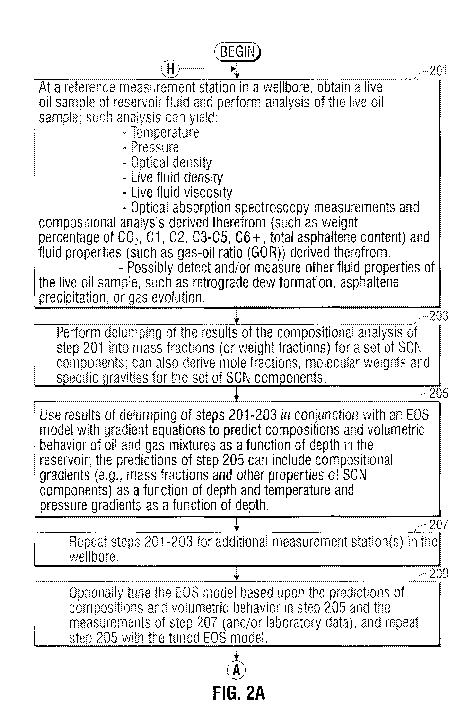
[0057] The operations of FIGS. 2A ._. 2G begin in. step 201 by employing the
downhole fluid
analysis (DFA) tool of FIGS. IA and lB to obtain a sample of the formation
fluid at the reservoir
pressure and temperature (a live oil sammple) at a measurement station in the
bvellbore (for
example, a reference station), The sample is processed by the fluid analysis
module 25. In the
preferred embodiment, the fluid :analysis module 25 performs spectrophotometry
measurements
that measure absorption spectra of the sample and translates such
spectrophot.ometry
measurements into concentrations of several alkane components and groups in
the fluids of
interest. In an illustrative embodiment, the fluid analysis module 25 provides
measurements of
the concentrations e.g., weight percentages) of carbon dioxide (CO2), methane
(CH4), ethane
(C2H6), the C3 C5 alkane group including propane, butane, pentane, the lump of
hexane and
27
CA 02772506 2012-02-27
WO 2011/030243 PCT/IB2010/053620
heavier alkane components (C6+), and asphaltene content. The tool 10 also
preferably provides
a means to measure temperature of the fluid sample (and thus reservoir
temperature at the
station), pressure of the fluid sample (and thus reservoir pressure at the
station), optical density
of the fluid sample, live fluid density of the fluid sample, live fluid
viscosity of the fluid sample,
gas-oil ratio (GOR) of the fluid sample, optical density, and possibly other
fluid parameters (such
as API gravity, formation volume fraction (FYF), etc.) of the fluid sample.
[0058] In step 203, a delumping process is carried out to characterize the
compositional
components of the sample analyzed in 201. The delumping process splits the
concentration (e.g.,
mass fraction, which is sometimes referred to as weight fraction) of given
compositional lumps
(C3-C5, C6-) into concentrations (e.g., mass fractions) for single carbon
number (SCN)
components of the given compositional lump (e,g., split C3-C5 lump into C3,
C4, CS, and split
(1'6+ lump into C6, C7, C8 ...). The exemplary de lumping operations carried
out as part of step
203 are described in detail in J.S. patent Application Publication
2009/0192768, herein
incorporated by reference in its entirety.
(0059] In step 2.05, the results of the delumping process of step 203 are used
in conjunction
with an equation of state (EOS) model to predict compositions and fluid
properties (such as
volumetric behavior of oil and gas mixtures) as a function of depth in the
reservoir. In. the
preferred embodiment, the predictions of step 205 include property gradients,
pressure gradients,
and to aperature gradients of the. reservoir fluid as a function of depth. The
property gradients
preferably include mass fractions, mole fractions, molecular weights and
specific gravities for a
set of SCN components (but not for asphaltenes) as a function of depth in the
reservoir. The
property gradients predicted in step 205 preferably do not include
compositional. gradients (i.e.,
m .ass fractions, mole fractions, molecular weights and specific gravities)
specifically for resins
"28
CA 02772506 2012-02-27
WO 2011/030243 PCT/IB2010/053620
and asphaltenes as a function of depth, as such analysis is provided by a
solubility model as
described herein in more detail. The variations of fluid properties with depth
represent the
variations of the bulk fluid (solution) properties, although resins and
asphaltertes are not
specifically treated.
[0060] The EQS yodel of step 205 includes a set of equations that represent
the phase
behavior of the compositional components of the reservoir fluid.. Such
equations can take many
forms. For example, they can be any one. of n. any cubic EOS, as is well
known. Such cubic
EQS include van der Waals FOS (1873), Redlich-Kwong EQS (1949), Soave-Redlich-
Kwong
EOS (1972), Peng-Robinson EQS (1976), Strvjek-Vora-Perng-Robirnso n EQS (1986)
and Patel-
Teja EOS (1982). Volume shift parameters can be employed as part of the cubic
EQS in order to
improve liquid density predictions, as is well known. Mixing rules (such as
van der Waals
mixing rule) can also he employed as part of the cubic EQS. A SAl~ l7-type EOS
can also he
used., as is well known in the art In these equations, the deviation from the
ideal gas law is
largely accounted for by introducing (1) a finite (non-zero) molecular volume
and (2) some
molecular interaction. These parameters are then related to the critical
constants of the different
clerical components.
(00611 In the preferred embodiment, the EQ=S model of step 205 predicts
compositional
gradients with depth that take into account the impacts of gravitational
forces, chemical forces,
thermal diffusion, etc. To calculate compositional gradients with depth in a
hydrocarbon
reservoir, it is usually assumed that the reservoir fluids are connected
(i.e., there is a lick of
compartmentalization) and in thermodynamic equilibrium (with no adsorption
phenomena or any
kind of chemical reactions in the reservoir). The mass flux (J) of
compositional component i that
crosses the boundary of an elementary volume of the porous media is expressed
as:
29
CA 02772506 2012-02-27
WO 2011/030243 PCT/IB2010/053620
{
when,, Li,- and L r are the phenomenological coefficients,
pi denotes the partial density of component i,
p, g, p, T are the density, the gravitational. acceleration, pressure, and
temperature, respectively, and
19I" is the contribution of component j to mass free energy of the fluid in a
porous media, which can be divided into a chemical potential part pi and a
gravitational
part gz (where z is the vertical depth).
[0062] The average fluid velocity (u) is estimated by:
fE (12)
p
[00631 According to Da.rcys law, the phenomenological biro-diffusion
coefficients must
meet the following constraint:
- f_I (13)
Ft P
where k and P. are the perryaeahility and the viscosity, respectively.
(00841 If the pore size is far above the mean free path of molecules, the
mobility of the
components, due to an external pressure field, is very close to the overall
mobility. The frnass
chemical potential is a function of rtaole fraction (x), pressure, and
temperature.
CA 02772506 2012-02-27
WO 2011/030243 PCT/IB2010/053620
[0065] At constant temperature, the derivative of the mass chemical potential
(j) has two
contributions:
axX
14)
Vr 'a"
VP
'IX where the partial derivatives can be expressed in terns of FOS (fugacity
coefficients):
i I` ` taa eta --
------ ---------
~)X Al X ax,
( + (16)
F_ x I} -, P 1~1 ai r'..r
where l'j, pj, and vi are the molecular mass, fugacity, fugacity coefficient,
and partial
molar volume of component j, respectively;
Xk is the mole fraction of component k;
R denotes the univer gal Pas constant; and
6 is the Kronecker delta function.
(0066] In the ideal case, the phenomenological coefficients (L) can be related
to effective
practical diffusion coefficients (Di"r5):
"I 0 7)
The mass conservation for component i in an ti-component reservoir fluid,
which governs the
distribution of the components in the porous media, is expressed as:
31
CA 02772506 2012-02-27
WO 2011/030243 PCT/IB2010/053620
t~jjFP. F
The equation can be used to solve a wide range of problems. This is a dynamic
model which is
changing with time t.
[0067] Let us consider that the mechanical equilibrium of the fluid column has
been
achieved.
V,P= (19)
[0068] The vertical distribution of the components can be calculated by
solving the following
set of equations
a In 11,,g ,Jii. M L;Q OT
t,z RT x, D pt 'M1 De" Dz
and
'a- ~,% -~'-.---- ---,-;- IM 7x, + $J-C-p--:----i fs ' `- ---' `'~. Fr 0 (2~.
3
kaf Xk q3, ax" x RI' x1D y p~IM, D Dz.
where Jj.i is the vertical component of the external mass flux and M is the
average
molecular mass. This formulation allows computation of the stationary state of
the, fluid
col nin and it does not require modeling of the dynamic process leading to the
observed
compositional distribution.
[0069] If the horizontal components of external fluxes are significant, the
equations along the
other axis have to be solved as well. Along a horizontal "x" axis the
equations become:
32
CA 02772506 2012-02-27
WO 2011/030243 PCT/IB2010/053620
a Int + .A* m - 4 a7' (22)
t
[0070] The mechanical equilibrium of tie fluid column V,P=pg, is a particular
situation
which will occur only in highly permeable reservoirs. In the general case, the
vertical Pressure
gradient is calculated by:
VP =.M- V., `Fri x-o-- r ,o rz (23)
z 1+ R,,
where R, is calculated by
#, =. `- --"--1----eft . (2.4)
F i=ED
[0071] The pressure gradient contribution from thermal diffusion (so-called
Soret
contribution) is given by:
1 1' .ff
[0072] And the pressure gradient contribution from external fluxes is
expressed as
(0073] Assuming an isothermal reservoir and ignoring the external flux,
results in the
following equation.
alay.. M- (27)
[0074] E q. (27) can be rewritten. as
33
CA 02772506 2012-02-27
WO 2011/030243 PCT/IB2010/053620
W ; = & = ,23..o4sa . (2$)
where aj is computed by:
I_ . M 'v,, t
XiDrlY phi EY' az
The first part of the a term of Eq. (29) can be simplified to
Ji" (30)
T he second part of the as term of Eq. (2-0) can be written in the form
proposed by Haase in
"Thermodynamics of Irreversible Processes,", ,kddison-- irYesley, Chapter 4,
1969. In this manner,
a, is computed by:
. Y + EW - . AT , i - :1,2,,.,, n (31)
xt :-,r M, M, T
ti
where H; is the partial molar enthalpy for component i; H, is the molar
enthalpy for the
mixture, Mr is the molecular mass for component i, Mm is the molecular mass
for the
mixture, T is the formation teramperature, and AT is the temperature
difference between
t io vertical depths.
The first part of the a3 terra of Eqs. (29) and (31) accounts for external
fluxes in the reservoir
florid. It, can be ignored if a steady state is assumed. The second part of
the aaa term of Ecls. (29)
and (31.) accounts for a temperature gradient in the reservoir fluid. It can
be ignored if an
isotlhernial reservoir is assurraed.
[0075] The fugacity,, of component i at a given depth can be expressed as
function of the
34
CA 02772506 2012-02-27
WO 2011/030243 PCT/IB2010/053620
fugacity coefficient and mole fraction for the component i and reservoir
pressure (P) at the given
depth as
The mole fractions of the components at a given depth must further sum to I
such that 1.. = I
at a given depth. Provided the mole fractions and the reservoir pressure and
temperature are
known at the reference station, these, equations can be solved for mole
fractions (as well as amass
fractions), partial r a.olar vokanes and volume factions for the reservoir
fluid components as well.
as pressure and temperature as a function of depth. Flash calculations can
solve for fugacities of
components (including the asphaltenes) that form at equilibrium. Details of
suitable flash
calculations are described by Li in "Rapid Flash Calculations for
Compositional Simulation,"
SPE Reservoir Evaluation and Engineering, October 2006, herein incorporated by
reference in its
entirety. The flash equations are, based on a fluid phase equilibria model
that finds the number of
phases and the distribution of species among the phases, that minimizes Gibbs
Free Energy.
More specifically, the flash calculations calculate the equilibrium phase
conditions of a mixture
as a function of pressure, temperature and composition. The fugacities of the
romponerats
derived. from such flash calculations can be used to derive asphaltene content
as a function of
depth employing the equilibrium equations described in U.S. Patent Application
Publication
20Oa=rt 2 7 1, herein incorporated by reference in its entirety.
[0076] In step 205, the predictions of compositional. gradient can be used to
predict
properties of the reservoir fluid as a function of depth (typically referred
to as. a property
gradient), as is well known. For example, the predictions of compositional
gradient can be used
CA 02772506 2012-02-27
WO 2011/030243 PCT/IB2010/053620
to predict bubble point pressure, derv point pressure, live fluid molar
volume, molecula weight,
gas-oil ratio, live fluid density, viscosity, stock tank oil density, and
other pressure-volume-
temperature (PVT) properties as a function of depth in the reservoir.
[0077] In step 207, the DFA too[ 10 of FIGS. IA mad IB is used to obtain a
sample of the
formation fluid at the reservoir pressure and temperature (a live oil sample)
at another
measurement station. in the wellborn, and the downhole fluid analysis as
described above with
respect to step 201 is performed on this sample. In an illustrative
embodiment, the fluid analysis
module 2.5 provides measurements of the concentrations (e.g., weight
percentages) of carbon
dioxide (C02), m Methane (Cl-l4), ethane (C-21-16), the .'3-C5 alkane group
including propane,
butane, pentane, the lump of hexane and heavier alkane components (C6-), and.
asphaltene
content. The tool 10 also preferably provides a means to measure temperature
of the fluid
sample (arid thus reservoir temperature at the station), pressure of the fluid
sample (and reservoir
pressure at the station can be obtained from pretest), live fluid density of
the fluid sample, live
fluid viscosity of the fluid sammple., gas-oi.l ratio (GOR) of the fluid
sample, optical density, and
possibly ether fluid parameters (such as API gravity, formation volume
fraction (FVF , etc.) of
the fluid sample.
[0078] Optionally, in stop 209 the EOS model of step '205 ca ::n he tuned
based on a
comparison of the compositional and fluid property predictions derived by the
EQ g model of
step 205 and the compositional and fluid property analysis of the DFA tool in
207. Laboratory
data can also be used to to .e the FOS model. Such tuning typically involves
selecting
parameters of the EQS model in order to improve the accuracy of the
predictions generated by
the EOS model. ELKS model parameters that can be tuned include critical
pressure, critical
temperature and acentric factor for single carbon components, binary
interaction coefficients,
36
CA 02772506 2012-02-27
WO 2011/030243 PCT/IB2010/053620
and volume translation parameters. An example of EOS model tuning is described
in .cyadh A.
Aimehaideb et aL, "EQS tuning to model full field crude oil properties using
nil.altiple well fluid
PVT analysis," Journal of Petroleum Science and Engineering., Volume 26,
Issues 1-4, pp. 291-
'500, 2000, herein incorporated by reference in its entirety. In the event
that the E OS model is
tuned, the compositional and fluid property predictions of step 205 can be
recalculated from the
turned EOS model.
[0079] In step, 211, the predictions of compositional gradients generated in
step 205 (or in
step 209 in the event that the EQS is tuned) are used to derive solubility
parameters of the,
solution (and possibly other: property gradients or solubility model inputs)
as a function of depth
in the oil column. For example, the predictions of compositional gradients can
he used to derive
the density of the solution (Eq. (2)). the molar volume of the solution (Eq.
(3)), and the solubility
parameter of the solution (1 q. (4) or (5)) as a function of depth,
[0080] In steps 213 to 219, the solute part is treated as a particular first-
type class, for
example a class where the solute part includes resins (with little or no
asphaltene nranoaggregates
and asphaltene clusters). This class generally corresponds to reservoir fluids
that include
condensates with very small concentration of asphaltenes. Essentially, the
high content of
dissolved gas and light hydrocarbons create a poor solvent for asphaltenes.
Moreover, the
processes that generate condensates do not tend to generate asphaltenes. For
this class, the
operations rely on an estimate that the average spherical diameter of resins
is 1..25 0.15 nm and
that resins impart color at a predetermined visible wavelength (e.g. 647 rim),
The average
spherical diameter of 1,25 0.15 urn corresponds to an average molecular weight
of 740 250
gr`n it. Laboratory centrifuge data also has shown the spherical diameter of
resins is hr 1..3 rnra.
This is consistent with the results in the literature. It is believed that
resins i.na.part color in the
37
CA 02772506 2012-02-27
WO 2011/030243 PCT/IB2010/053620
shorter visible wavelength range due to their relatively small number of fused
aromatic rings
("FARs") in polycyclic aromatic hydrocarbons ("PAHs"). In contrast,
asphaltenes impart color
in both the short visible wavelength range and the longer near-infrared
wavelength range due to
their relatively larger number of PARS in PAIs. Consequently, resins and
asphaltenes impart
color in the same visible wavelength range due_ to overlapping electronic
transitions of the
numerous PAHs in the oil. However, in the longer mar-infrared wavelength
range, the optical
absorption is predominantly due to asphaltenes.
[0081] In step 215, a number of average spherical diameter values within the
range of
1..25 O.15 nrn (e.g., d = 1.1 nm, d=1.2 m, d=1.3 nm and d=L4 nm) are used to
estimate
corresponding molar volumes for the particular solute part class utilizing E
q. (9).
(0082] In step 211, 7, the molar vohrrnes estimated in step 215 are used in
Conjunction with the
Flory-Huggins type model described above with respect to Eq. (1) to generate a
family of curves
that predict. the concentration of the particular solute part class of step
21:3 as a function of depth
in the reservoir.
[00831 In step 219, the family of curves generated in step 217 are compared to
measurements
of resin concentration at corresponding depths as derived from associated DFA
color
measurements at the predetermined visible wavelength (647 nm). The comparisons
are
evaluated to identify the diameter that best satisfies a predetermined
matching criterion. In the
preferred embodiment, the matching criterion determines that there are small
differences
between the resin concentrations as a function of dept) as predicted by the
Flory- Uuggins type
model and the corresponding resin concentrations measured from. DFA analysis,
thus providing
an indication of a proper match within an acceptable tolerance level.
38
CA 02772506 2012-02-27
WO 2011/030243 PCT/IB2010/053620
[0084] In steps 221 to 227, the solute part is treated as a particular second-
type class, for
example a class where the solute part includes asphaltene nanoagg-regates
(with little or no resins
and asphaitene clusters,). This class generally corresponds to low GOR black
oils that usually
have little conipr"e ssibility. These types of black oils often contain
asphaltene molecules with 4
to 7 FAR.s in PAl-Is. The asphaltene molecules are dispersed in the oil as
narnoa gregates with an
aggregation rmmher of 2-8. For this class, the ope-ations rely on an estimate
that the average
spherical diameter of a-sphaltene nanoaggregates is L 8 M aura and that the
asplhaltene
nanoaggregates impart color at a predetermined near-infrared (NIR) wavelength.
(e.g. 1070 nrrr),
The average spherical diameter of 1,8 0.2 rim corresponds to an average
molecular weight of
2200 700 g/m.ol. This is consistent with the results i the literature. Field
and laboratory
analysis have shown that asphaltene nanoaggregates impart color in both the
visible wavelength
range around d40 nrrm and the NIR wavelength range around 1070 rim. It is
belie-vied that the
asphaltene nanoaggegates impart color in both the short visible wavelength
range and the longer
near-infrared wavelength range due to their relatively larger number of FARs
in PAHs.
[0085] in step 223, a number of average spherical diameter values within the
range of
1, 8 -0.2 tine (e- g, d = 1.6 nn, d=1.7 nm, d=1.8 nm, d=l .9 nm and d= 2.0 nn)
are used to estimate
corresponding molar volumes for the particular solute part class utilizing Eq.
(9).
[0088] In step 225, the molar volumes estimated in step 223 are used in
conjunction with the
Tory-Hug ins type model described above with respect to Eq. (1) to generate a
family of curves
that predict the concentration of the particular solute part class of step 221
as a function of depth
in the reservoir,
[0087] In step 227, the fancily of curves generated in step 225 are compared
to measurements
39
CA 02772506 2012-02-27
WO 2011/030243 PCT/IB2010/053620
of asphalterae naraoaggregate Concentration at corresponding depths as derived
from associated
DFA color measurements at the predetermined NIR wavelength (1.070 m). The
comparisons
are evaluated to identify the diameter that best satisfies a predetermined
matching criterion. In
the preferred embodiment, the. matchin criterion determines that there are
small differences
between the asphaltene narroaggre gate concentrations as a function of depth
as predicted by the
Flory-Huggins type model and t .e corresponding asphaitene nanoaggregate
concentrations
measured from DFA analysis, thus providing an indication of a proper match
within an
acceptable tolerance level.
[OQ88] In steps 229 to 23 5, the solute part is treated as a particular third-
type class, for
example a class where the solute part includes a combination of resins and
asphaaltene
nanoaggregates (with little or no asphaltene clusters). This class generally
corresponds to black-
oils that include a mixture of resins and asphaltene nanoaaggregates. For this
class, the operations
rely on an estimate that the average spherical diameter of the remixed resins
and asphaa.ltene
nanoaggregates varies linearly from 1.5 0.2 am to 2,0 0.2 nm according to
wavelength in -a
range between a visible wavelength (647 nrn) and a NIR wavelength (1070 urn).
This conforms
to an assumption that the average molecular diameter for r nixed resin and
asphaltene
naraoaggeg;rates increases linearly with increasing wavelength due to the
increasing importance
of absorption from the asphaltene aggregates in the longer wavelength region.
It is believed that
the asphaltene nauoaggregate content (weight percent) contributin to color
increases
exponentially with increasing wavelength. in the preferred embodiment, the
relationship
between the average spherical diameter (d) and wavelength can be given by:
d = C I *Wavelength + C2 (33)
where C I and C2 are constants.
CA 02772506 2012-02-27
WO 2011/030243 PCT/IB2010/053620
C I and C21 can be determined by solving the relation utilizing two
diameter/wavelength
combinations. For instance, a combination of d = 1.5 as at 647 am wavelength
and. a
combination of d = 2.0 am at 1070 area wavelength can be used to solve for Cl
and C2. In
:ano -her example, a combination of d = 1.3 urn at. 647 as:an wavelength and a
combination of d
1.8 run at 1070 ram wavelength can be used to solve for Cl and C2. In yet
another example, a
combination of d = 1.7 am at 647 nm wavelength and a combination of d. = 2.2
ram at 1070 tarn
wavelength can be used to solve for C I and C2.
[0089] In step 221, a number of average spherical diameter values and
wavelength
combinations defined by the relationship of step 229 are used to estimate
corresponding molar
volumes for the particular solute part class utilizing Eq. (9),
[0090] In step 233, the molar volumes estimated in step 231 are used in
conjunction. with the
Flory-Huggins type solubility model described above with respect to Eq. (1) to
generate a family
of curves that predict the concentration of the particular solute part class
of step 229 as a function
of depth in the reservoir. Each curve is associated with a particular average
spherical diameter
value and wavelength combination.
[0091] In. step 235, the family of curves generated in step 233 are compared
to measurements
of mixed resins and asphaltene nanoaggregate concentrations at corresponding
depths as derived
from ass aciated DFA color measurements at the wavelength of the given dia
titer/wav'elength
combination for the respective curve. The comparisons are evaluated to
identify the diameter
that best satisfies a predetermined matching criterion. In the preferred
embodiment, the
matching criterion determines that, there are small differences between the
mixed resin and
asphaltene_ nanoaggregate concentrations as a function of depth as predicted
by the Flory-
4 1
CA 02772506 2012-02-27
WO 2011/030243 PCT/IB2010/053620
Huggins type model and the corresponding mixed resin and asphaltene nanoaggg
negate
concentrations measured from DFA analysis, thus providing an indication of a
proper match
,within an acceptable tolerance level,
[0092] In steps 237 to 243, the solute part is treated as a particular fourth-
type class, for
example a class where the solute part includes asphaltene clusters. This class
generally
corresponds to black oils where the asphaltene gradient is very large in the
oil column. This
behavoir implies that both asphaltene nanoaggregates and asphalene clusters
are suspended in the
oil column. For this class, the operations rely on an estimate that the
average spherical diameter
of asphaltene clusters is 4.5 0.5 nay. at. a predetermined NIR wavelength
(1070 inn). field and
laboratory analysis have shown that asphaltene clusters impart color in both
the visible
wavelength range around 640 um and the NIR wavelength range around 1070 nn. It
is believed
that the asphaltene clusters impart color in both the short visible wavelength
range and the longer
NLR wavelength range due to their relatively larger number of PARS in PAI-Is.
[0093] In step 239, a number of average spherical diameter values within. he
range of
4,5"_U nm (e.g., d = 4.0 nna., d=4.3 urn, drn4.5 urn, d=4.8 mu arid (1=5.0
nrn) are used to estimate
corresponding molar volumes for the particulars solute part class utilizing E
q, (9).
[0094] In step 241, the molar volumes estimated in step 239 are used in
conjunction with the
Flory-Huggins type model described above with respect to Eq. (1) to generate a
family of curves
that predict the concentration of the particular solute part, class of step
237 as a function of depth
in the reservoir.
[0095] In step 243, the family of curves generated in step 241 are compared to
measurements
of asphaltene cluster concentration at corresponding depths as derived from
associated DFA
42
CA 02772506 2012-02-27
WO 2011/030243 PCT/IB2010/053620
color measurements at the predetermined NIR wavelength (1.070 urn). The
comparisons are
evaluated to identify the diameter that best satisfies a predetermined
matching criterion. In the
preferred embodiment, the matching criterion determines that there are small
differences
between the asphaltenr cluster concentrations as a function of depth as
predicted by the Flory-
Huggins type model and the corresponding asphaltene cluster concentrations
measured from
DFA analysis, thus providing an indication of a proper match within an
acceptable tolerance
level.
[0096] In step 245, the matching diameter's identified in steps 219, 227, 235
and 243 (if any)
are evaluated to determine the best matching diameter of the group. The
evaluation provides an
indication of which particular solute part class (and thus the assumption Of
Composition
underlying the particular solute part class) is the best match to the measured
gradient for the.
solvent part compositions,.
[0097] In step '247, the result of the evaluation of step 245 is analyzed to
determine if the best
to atching diameter corresponds to the solute part class of steps 213 co 219
where the solute part
includes resins (with little or no asphaltene naanoaggregates and asphaltene
clusters). If the
answer is yes, the operations Continue to step 249. Otherwise the operations
continue to step
251.
[0098] In step 249, the workflow declares that that the reservoir fluids are
in thermal
equilibrium within a non-compartmentalized reservoir, and the reservoir fluids
include resins
(with little or none asphaltene nanoag regates or asphaltene clusters) in
accordance with
assumptions underlying the solute part class of steps 213 to 219. In this
case, the reservoir fluid
includes condensates with a very small concentration of asphaltenes.
Essentially, the hi a
43
CA 02772506 2012-02-27
WO 2011/030243 PCT/IB2010/053620
content of dissolved gas and light hydrocarbons create a very poor solvent for
asphaltenes.
Moreover, processes that generate condensates do not tend to generate
asphaltencs.
Consequently, there is very; little. crude oil color as determined by DFA in
Elie near-infrared
range Nevertheless, there are asphaltene like u .olecules -the resins --- that
absorb visible light
and at times even some near infrared. light. These resin molecules are largely
dispersed in the
condensate as molecules - thereby reducing the impact of the gravitational
terns. In addition,
condensates exhibit considerable gradients. Since condensates are
compressible, the hydrostatic
head pressure of the condensate colurrm generates a density gradient in the
column. The density
gradient creates the driving force to create a chemical composition gradient.
The lower density
components tend to rise in the column while the higher density components tend
to settle down
in the column. This GO R gradient gives rise to a large solubility contrast
for the resins, thereby
producing s g;aificant DFA color gradients. These gradients are useful to
check for reservoir
connectivity. Accordingly, the GOR gradient as determined by DFA analysis can
be evaluated
for reservoir analysis, The predicted and/or measured concentration of the
resin component as a
function of depth can also be evaluated for reservoir analysis. More
specifically, connectivity
can be indicated by moderately decreasing G-OR values with depth, a continuous
increase of
resin content as a function of depth, and/or a continuous increase of fluid
den ity ar d/ora fluid
viscosity as a function of depth. On the other hand, compartmentalization
and/or non
equilibrium can be indicated by discontinuous C_aOR (or if lower CIOR is found
higher in the
column), discontinuous resin content (or if higher a-sphaltere content is
fowid higher in the
colun.m), and/or discontinuous fluid density and/or- fluid viscosity (or if
higher fluid density
and/or fluid viscosity is found higher in the coluunin).
[00991 In step 2.51, the result of the evaluation of step 245 is analyzed tee
determine if the best
44
CA 02772506 2012-02-27
WO 2011/030243 PCT/IB2010/053620
matching diameter corresponds to the solute part class of steps 221 to 227
where the solute part
includes asphaltene nanoaggregates (with little or no resins and asphaltene
clusters). If this is the
case, the operations continue to step 253. Otherwise the operations continue
to step 255.
[00100] In step 253, the workflow declares that the reservoir fl rids are in
thermal
equilibrium within a non-comm.partrmrttalired reservoir, and the resetwoir
fluids include
asphaltene nanoags egates (with little or no resins and asphaltene clusters)
in accordance with
assumptions underlying the solute part class of steps 221 to 2'2 where the
solute part includes
asphaltene nanoag
_Wegates (with little or no resins and aspha.lterr : clusters). In this case,
the
predicted and/or measured concentration of the asphaltene nanoaggregates as a
function of depth
can he evaluated for reservoir analysis, More specifically, connectivity can
be indicated by a
continuous increase of asphaltene nanoaggregate content as a function of
depth, and/or a
continuous increase of fluid density and/or fluid viscosity as a function of
depth. On the other
hand, comp~rrt ~rertital.i at.ion anad/or non-equilibrium can be indicated by
discontinuous asphaltene
nanoaggregate content (or if higher asphaltcne nanoaggreage content is found
higher in the
column), and/or discontinuous fluid density and/or fluid viscosity (or if
higher fluid density
and/or fluid viscosity is found higher in the column.).
[00101 In step 255, the result of the evaluation of step 245 is analyzed to
determine if the
best matching diameter corresponds to the solute part class of steps 229 to
235 where the solute
part includes a mix of resins and asphaltene nanoaggregates (with little or no
asphalte--ne
clusters). If this is the case, the operations continue to step 257. Otherwise
the operations
continue to step `2.59.
(00102] In step 257, the workflow declares that the reservoir fluids are in
thermal
CA 02772506 2012-02-27
WO 2011/030243 PCT/IB2010/053620
equilibrium ,Within a non-compartmentalized reservoir, and the reservoir
fluids include, a rixtu:`e
of resins and asphaltene nanoaggre aÃes (with little or no asphalt n in
accordance with
assurnpiio s underlying the solut,. part class of steps 229 to 235 ,-here the
solute part includes a
mixture of resins and asphaliene rna oaaggregates (with little or no asp
altene clusters). In this
ease, the- predicted and/or measured concentration of the mixtur : of resins
and asphaltene
. eeificali 9
nan aggregates as a function of depth can be evaluated fat reservoir analysis.
More,
corttaea: tivity can be indicated b r a continuous increase of the
concentration of the
re iin/asphaltene nanoag regate mixture as a fu .ction of depth, and/or a
continuous increase of
fl,tui.di density anti/or fluid viscosity as a function cif depth. On the
other hand,
co mpartine atalization and/or non-equiJ:iUdurn can be indicated by
discontinuous concentration of
the resin/asphaitene nanoaggregate mixture (or if a higher concentration of
the resiniasphaltene
udn oaggreage m i.xture is found higliet in the Column), and/or discontinuous
fluid density and/or
fluid viscosity (or if higher fluid density and/or, fluid viscosity is found
higher in the column).
[0010 ] In step 259, the result of the evaluation of step 245 is analyzed to
determine if the
best matching diameter corresponds to the solute part class of steps 237 to
243 where the solute
part includes asphalterne clusters. If this is the case, the operations
continue to step 261.
Otherwise the operations continue to step 263.
[00104] In step 261, the Workflow declares that the reservoir fluids are in
thermal
egdIibriun within a non-eoinpartznentalizcd reservoir; and the reset on fluids
include
asphaltene clusters in accordance with assumptions underlying the solute part
elas, of steps 237
to 243 where the solute part includes asphaltene clusters, fn this case, the
predicted and/or
measured concentration of the asphaltene clusters as a function of depth can
be evaluated for
reservoir analysis. More specifically, connectivity can be ind by a continuous
increase of
46
CA 02772506 2012-02-27
WO 2011/030243 PCT/IB2010/053620
asphaltene cluster content as a function of depth, and/or a continuous
increase of fluid density
and/or fluid viscosity as a function of depth. On the other hand,
cornpartmenta(ization and/or
non-equilibrium can be indicated by discontinuous asphaltene cluster content
or if higher
asphalten . cluster content is found higher in the column), and/or
discontinuous f4 rid, density
andl/or fl aid viscosity (or if higher fluid density andior fluid. viscosity
is found higher in the
column. Morever, because asphaltene clusters are expected in the oil colur, it
is anticipated
that:
- large density and viscosity gradients exist in the oil column;
- the oil may have flow assurance problems (due to instabilty from e.g., the
asphaltene
onset pressure being equal to or greater than the formation pressure, or
bitumens in
the formation); and
- there may be an alloclithouous tar mat in the reservoir (as opposed to an
autochdionous tar mat formed from biodegradation).
[00105] In step 263, no suitable match has been found between the solubility
curves and
the measured properties. In this case, the operations can determine if there
is a need for
additional measurement stations and/or different methodologies for repeat
processing and
analysis in order to improve the confidence level of the measured arid/or
predicted fluid
properties. For e xaniple, the measured and/or predicted properties of the
reservoir fluid can be
compared to a database of historical reservoir data to determine whether the
measured and/or
predicted properties make sense. If the data does not make sense, additional
measurement
station(s) or different methodologies (e.g., different model(s)) can be
identified for repeat
processing and analysis in order to improve the confidence level of the
measured acid/or
47
CA 02772506 2012-02-27
WO 2011/030243 PCT/IB2010/053620
predicted fluid properties.
[00106] Other factors can be used to determine if there is a need for
additional
measurement stations and/or different methodologies for repeat processing and
analysis in order
to improve the confidence level of the measured and/or- predicted fluid
properties. For example,
in step 263, it is expected that the reservoir is compartmentalized or not in
thermodynamic
equilibrium. Thus, the measured fluid properties can be accessed to confirm
that they
correspond to this expected architecture.
[00107] If in step 263 there is a need for additional measurement stations
and/or different
methodologies, the operations continue to step 265 to repeat the appropriate
processing and
analysis in order to improve the confidence level of the measured and'or
predicted fluid
properties.
[00108] If in step 263, there is no need for additional measurement stations
and/or
different methodologies (in other words, there is sufficient confidence level
in the measured
and/or predicted fluid properties), the operations cont.i .t.re to step 267
where the reservoir
architecture is determined to be compartmentalized and/or not in thermodynamic
equilibrium.
Such a determination is supported by the invalidity of the assumptions of
reservoir connectivity
and thermal equilibrium that underlie the models utilized for predicting the
solute part property
gradient within the wellbore.
[00109] Subsequent to the determination of reservoir architecture in steps
249, 253, 257,
261., and 267, the results of such determination are reported to interested
parties in step 269. The
characteristics of the reservoir architecture reported in step 269 can be used
to model and/or
understand the reservoir of interest for reservoir assessment, planning, and
management..
48
CA 02772506 2012-02-27
WO 2011/030243 PCT/IB2010/053620
[0011 There have been described and illustrated herein a preferred embodiment
of a
method, system, and apparatus for downhole fluid analysis of the fluid
properties of a reservoir
of interest and for characterizing the reservoir of interest. based upon such
downhole fluid
analysis. While particular embodiments of the invention have been described,
it is not intended
that the invention be limited thereto, as it is intended that the invention be
as broad in scope as
the art will allow and that the specification be read likewise. Thus, while
particular equations of
state models, solubility models and applications of such models have been
disclosed for
predicting properties of reservoir fluid., it will be appreciated that other
such models and
applications thereof could be used as well. Moreover, the methodology
described herein is not
limited to stations in the same weilbore, For example, measurements from
samples from
different wells can be analyzed as described herein for testing for lateral
connectivity. In
addition, the workflow as described herein can be modified, For example, it is
contemplated that
user input can select the solute type classes from a list of solute type
classes for processing. The
user might also be able to specify certain parameters for the processing, such
as diameters that
are used as input to the solubility model to derive concentration curves for
the relevant solute
part classes, as well as optical density wavelengths that are used to
correlate such concentrations
to concentrations measured by dowialaole fluid analysis, It will therefore be
appreciated by those
skilled in the art that yet other modifications could be made to the provided
invention without
deviating from its scope as claimed.
49