Note : Les descriptions sont présentées dans la langue officielle dans laquelle elles ont été soumises.
CA 02817104 2013-05-06
WO 2012/065267 PCT/CA2011/050710
METHODS AND APPARATUS FOR ALIGNMENT OF INTERFEROMETER
CROSS-REFERENCE TO RELATED APPLICATION
This application claims priority to U.S. Provisional Application No.
61/414,044, titled "AUTOMATIC INTERFEROMETRIC ALIGNMENT OF AN
OPTICAL COHERENCE TOMOGRAPHY SYSTEM" and filed on November 16th,
2010, the entire contents of which are incorporated herein by reference, and
to
U.S. Provisional Application No. 61/434,924, titled "METHOD AND APPARATUS
FOR ALIGNMENT OF INTERFEROMETER" and filed on January 21st, 2011, the
entire contents of which are incorporated herein by reference.
BACKGROUND
This disclosure relates to methods and apparatus for stabilizing free space
interferometry systems. More particularly, this disclosure relates to methods
and
apparatus for stabilizing optical coherence tomography systems employing free
space interferometry.
Optical Coherence Tomography (OCT) is a quickly advancing
interferometric medical imaging technology that allows for high-resolution and
non-destructive tomographic imaging. One of its primary current uses is for in
vivo and ex vivo examination of medical samples, and is often used to study
ocular, vascular, respiratory, dental, dermal, neurological, and
gastrointestinal
diseases. OCT fills an imaging niche between low resolution, high penetration
depth imaging techniques like ultrasound (US) and magnetic resonance imaging
(MRI) modalities and high resolution, low penetration techniques like confocal
1
CA 02817104 2013-05-06
WO 2012/065267 PCT/CA2011/050710
microscopy (CM) techniques. OCT provides high resolution imaging (-1 pm) over
3D volumes spanning several millimeters with minimal sample preparation time.
Some primary advantages of OCT imaging include rapid imaging of biological
tissue with minimal sample preparation, 3D high-resolution imaging with depth
penetrations of several millimeters, and the capability to obtain results in
real
time, and allowing for fast and minimally invasive identification of many
diseases.
Currently, there is often a significant hurdle between state-of-the-art
research systems and commercial implementations of OCT systems. In
particular, many high end research systems use a free-space optical design
that
may necessitate frequently stopping to realign the system or special technical
expertise to operate the system. Such drawbacks can severely disrupt
productivity, and are typically avoided by reconfiguring the system design
using
fiber optic components to satisfy the reliability needs of a commercial
product.
This reconfiguration greatly improves the robustness of the system to
external effects but comes at the cost of additional development time and can
often reduce the overall system performance. The reconfigured system depends
on the robustness of the fiber to maintain system performance in variable
environmental conditions, but sacrifices the performance and flexibility of
free-
space optical designs.
The aforementioned sacrifice in system performance arises from the
inherent limitations of fiber optic components. Fiber optics are primarily
designed
for conveniently transporting light long distances. While very useful for OCT
systems, the available optical components and operating wavelengths are
2
CA 02817104 2013-05-06
WO 2012/065267 PCT/CA2011/050710
heavily limited compared to free-space choices. Current OCT systems implement
significant portions of their design in free-space optics, such as the sample
focusing system, because of these limitations. The fiber optics are primarily
used
in the interferometer body, where tolerances are most strict. Unfortunately,
by
enclosing the light transport path inside a fiber, it can be difficult to
modify and
enhance an already designed system.
In addition to the limitations in component choices, there can be
performance penalties for a fiber based design. Simple off-the-shelf fiber
cables
quote losses of 0.3 dB (-6.7%) compared with coated off-the-shelf free space
optical losses of less than 1%. In addition, coupling between free-space and
fiber
based systems, as performed in most current OCT systems, imposes additional
losses that can become fairly severe with minimal misalignment. Fiber optics
also
suffer from poorer control of polarization than free space optics. In order to
achieve a strong interference signal, maintaining proper polarization is
important.
While careful design and polarization controlling devices can mitigate some of
this effect in fiber systems, a free-space optical design makes polarization
control
much simpler. This can be especially important in polarization sensitive OCT
applications, such as Mueller OCT systems.
The chromatic variation in the index of refraction of fiber is also
substantially different and more significant than that of air, making it
important to
closely match the length of fiber in each arm of the interferometer to
minimize
dispersive effects. Because the path lengths in the interferometer already
need to
be closely matched in an OCT system, the removal of the fiber reduces this
3
CA 02817104 2013-05-06
WO 2012/065267 PCT/CA2011/050710
additional source of dispersion in the system.
With current trends in OCT technology, higher resolution systems are a
large focus of research. This requires extremely broadband light sources to
improve the axial resolution of the system. Because the wavelength range that
can efficiently propagate through a single mode fiber is constrained by the
physical parameters of the fiber, it can be difficult to design a fiber system
that
provides high throughput with a large spectral bandwidth. This can be
especially
difficult at short wavelengths, where high lateral resolution can also be
achieved.
By removing the fiber from the system, standard broadband optical coatings can
be used to provide high throughput over large wavelength regions.
One of the main advantages of fiber based designs is the ability to contain
large optical paths in an easily manipulated fiber. It is relatively simple to
encapsulate many meters of path length in a small coil that can be later
stretched
a long distance and then coiled again. A free-space optical system likely
needs to
be larger to accommodate the same path length requirements.
In a free-space system, efficiently travelling long distances can be difficult
and can greatly magnify small alignment errors¨a small tilt of a beam entering
a
fiber will cause a small light loss at the far end of the fiber while the same
error in
a free-space system could be magnified to a fairly large beam shear.
The discrete optics in a free-space system are also more sensitive to
positional effects. If a lens moves by a small amount, the beam position and
tilt
can change by relatively large amounts. These effects are both seen in
construction and in use and require special care in interferometric systems.
4
CA 02817104 2013-05-06
WO 2012/065267 PCT/CA2011/050710
Accordingly, the initial alignment of an interferometer built with free-space
optics
is significantly more difficult than a fiber based design. Temperature changes
of a
few degrees are sufficient to cause noticeable alignment changes and can occur
simply from the body heat of an operator near the system.
SUMMARY
Methods and apparatus are provided for the alignment of an
interferometric system. In one embodiment, a spatial filter comprising a
reflective
pinhole is provided at the output of the interferometer, and tilt is measured
by a
tilt detection subsystem positioned to reimage the pinhole. A shear detection
subsystem is positioned to image an offset of the interferometer beams. Tilt
and
shear offsets are determined by comparing measurements obtained from the tilt
and shear subsystems with pre-recorded measurements obtained for an aligned
state. The tilt and shear offsets are employed to realign the system using
positioning controls corresponding a reduced number of dominant degrees of
freedom of the system.
In one aspect, there is provided an alignment apparatus for aligning an
interferometer, wherein the interferometer is configured to separate and
recombine a first beam and a second beam in free space, and wherein a
misalignment of the interferometer is characterized by a reduced set of
dominant
degrees of freedom, the alignment apparatus comprising: for each dominant
degree of freedom: detection means for detecting an alignment associated with
the dominant degree of freedom and for providing an error signal associated
with
5
CA 02817104 2013-05-06
WO 2012/065267 PCT/CA2011/050710
the dominant degree of freedom; and a positioning element operatively
connected to the interferometer and configured to vary the alignment
associated
with the dominant degree of freedom; and a controller configured to control
each
positioning element and maintain alignment of the interferometer based on the
error signals obtained from the detection means.
In another aspect, there is provided an apparatus for aligning an
interferometer, the interferometer configured to separate and recombine a
first
beam and a second beam in free space, the apparatus comprising: a spatial
filter
located at an output of the interferometer, the spatial filter including a
focusing
optical element and a reflective optical element including a pinhole; a tilt
detection subsystem configured to reimage the pinhole for measuring a tilt of
the
first beam and the second beam; a shear detection subsystem configured to
image an offset of the first beam and the second beam for measuring a shear of
the first beam and the second beam; and two or more positioning elements
configured to vary a tilt and shear of the first beam and the second beam.
In another aspect, there is provided a method of aligning an
interferometric system, the interferometric system including an interferometer
and
an alignment apparatus according to claim 13, wherein the positioning elements
of the alignment apparatus are provided to compensate for errors resulting
from
a reduced set of dominant degrees of freedom for the interferometer, such that
one positioning element is provided for each reduced dominant degree of
freedom; the method comprising the steps of: a) determining a tilt offset from
the
tilt detection system; b) controlling at least one of the positioning elements
to
6
CA 02817104 2013-05-06
WO 2012/065267 PCT/CA2011/050710
correct for the tilt offset; c) determining a shear offset from the shear
detection
system; and d) controlling at least one of the positioning elements to correct
for
the shear offset.
A further understanding of the functional and advantageous aspects of the
disclosure can be realized by reference to the following detailed description
and
drawings.
BRIEF DESCRIPTION OF THE DRAWINGS
Embodiments will now be described, by way of example only, with
reference to the drawings, in which:
Figure 1 provides a schematic of the OCT system, showing the main
optical components, and the two sample and backend additional subsystems.
Figure 2 is a schematic of the sample scanning subsystem.
Figure 3 is a schematic of the spectrometer backend subsystem.
Figure 4 provides a series of images showing a comparison of the
returned signal from a mirror in the focal plane of the sample arm and a
representative scattering sample. Note the greatly increased size of the spot
returning from the sample and the residual light from a mirror spot that does
not
pass through the pinhole.
Figure 4(a) shows the focused spot from a mirror, with reduced exposure
time to avoid saturation.
Figure 4(b) shows the focused spot from a mirror.
Figure 4(c) shows focused spot from a mirror through the pinhole.
7
CA 02817104 2013-05-06
WO 2012/065267 PCT/CA2011/050710
Figure 4(d) shows the focused spot from the sample.
Figure 4(e) shows the focused spot from the sample through the pinhole.
Figure 5 provides images showing the ability to measure tilt
misalignments using the system. The images on the top show the measured
offset of the tilt while the plots on the bottom show the signal obtained at
the
detector. The cross near the image center indicates where the spot should be
while the other cross centroids the actual spot. The images on the top are
zoomed in views of the tilt sensor and do not show the full field of view.
Figure 6 provides images that show the ability to measure shear
misalignments using the system. The images on the top show the measured
offset of the shear while the plots on the bottom show the signal obtained at
the
detector. The images are heavily enhanced to highlight the edges in printed
form.
Note that this axis of control only affects the reference arm of the
interferometer
and so the signal from the sample arm is always present at the same intensity
in
the plots.
Figure 7 is a flow chart illustrating a method of automatically aligning an
interferometric system.
Figure 8 illustrates the effect of mirror shifts on a collimated beam, where
(a) shows an assumed initial configuration while (b) through (d) show the
effects
of offsets from this configuration. Solid light grey indicates the collimated
beam.
The solid rectangle shows the mirror position and orientation while the solid
line
shows the mirror normal from the center of the mirror. If needed, a dotted
line
shows the mirror normal at the incident point. Where appropriate, equivalent
8
CA 02817104 2013-05-06
WO 2012/065267 PCT/CA2011/050710
objects in dark highlight differences from the initial configuration.
Figure 9 illustrates the effect of various lens shifts, where (a) shows an
assumed initial configuration while (b) through (e) show the effects of
offsets from
this configuration. Solid light grey indicates collimated beams and light grey
lines
show focusing light. The oval shows the lens position and orientation while
the
rectangle shows the focal plane of the lens. Where appropriate, equivalent
objects in dark grey highlight differences from the initial configuration.
Figure 10 provides an optical layout to illustrate the adaptation of the
method to a wide range of interferometric devices. Black arrows indicate the
direction of light propagation.
DETAILED DESCRIPTION
Various embodiments and aspects of the disclosure will be described with
reference to details discussed below. The following description and drawings
are
illustrative of the disclosure and are not to be construed as limiting the
disclosure.
Numerous specific details are described to provide a thorough understanding of
various embodiments of the present disclosure. However, in certain instances,
well-known or conventional details are not described in order to provide a
concise discussion of embodiments of the present disclosure.
As used herein, the terms, "comprises" and "comprising" are to be
construed as being inclusive and open ended, and not exclusive. Specifically,
when used in the specification and claims, the terms, "comprises" and
"comprising" and variations thereof mean the specified features, steps or
9
CA 02817104 2013-05-06
WO 2012/065267 PCT/CA2011/050710
components are included. These terms are not to be interpreted to exclude the
presence of other features, steps or components.
As used herein, the term "exemplary" means "serving as an example,
instance, or illustration," and should not be construed as preferred or
advantageous over other configurations disclosed herein.
As used herein, the terms "about" and "approximately", when used in
conjunction with ranges of dimensions of particles, compositions of mixtures
or
other physical properties or characteristics, are meant to cover slight
variations
that may exist in the upper and lower limits of the ranges of dimensions so as
to
not exclude embodiments where on average most of the dimensions are satisfied
but where statistically dimensions may exist outside this region. It is not
the
intention to exclude embodiments such as these from the present disclosure.
Embodiments disclosed herein provide methods and apparatus that allow
the automatic monitoring and control of the alignment of an interferometric
optical
system, enabling practical, rugged and commercial free space interferometric
optical systems that deliver performance similar to customized research
systems
without requiring the use of fiber optics. Systems incorporating the methods
and/or apparatus of the present embodiments can be adapted to support high
throughput and allow for significant system customization. In particular,
embodiments provided below may enable the automatic control of alignment
without any user interaction over a large thermal range, and can further
compensate for misalignments during initial system construction or resulting
from
shock events. Accordingly, such systems may deliver controlled optical
stability
CA 02817104 2013-05-06
WO 2012/065267 PCT/CA2011/050710
with minimal interruption to a normal user's workflow.
The forthcoming disclosure illustrates embodiments involving the non-
limiting example of an OCT system. The basic principles of an OCT system are
first described, after which embodiments providing methods and apparatus are
disclosed whereby a free space OCT system is adapted for automated stability
control.
The example system described below is a free space OCT interferometer
that can automatically maintain its alignment, allowing for the use of a free-
space
optical design outside of tightly controlled laboratory environments. The
system
supports shortened OCT imaging times by increasing first-time accuracy of the
scan, removing artifacts and other effects that can compromise the resolution
of
the scan. The system corrects for small to moderate misalignments caused by
temperature fluctuations, shock events, and other perturbations. Selected
embodiments also provide minimally invasive monitoring and correction
hardware enhancements along with methods of calibrating this hardware for
improved performance.
While selected embodiments disclosed below relate to high-performance
medical interferometric imaging devices such as OCT devices, it is to be
understood that the scope of the embodiments disclosed herein is not to be
limited to such heuristic and non-limiting examples. The proceeding
embodiments may be readily adapted to a wide range of free space
interferometric devices. Furthermore, although the embodiments provided herein
relate to free space interferometric systems, it is to be understood that
systems
11
CA 02817104 2013-05-06
WO 2012/065267 PCT/CA2011/050710
according to the embodiments disclosed below may also include non-free-space
(i.e. optically guided) elements, provided that at least a portion of the
system
involves free space propagation between optical components. For example, an
interferometric optical system according to embodiments provided herein may
include a free space interferometric subsystem that connects to a guided
subsystem for a portion of the optical path, such as a free space
interferometer
having in its sample arm a guided optical subsystem such as a catheter housing
an optical fiber.
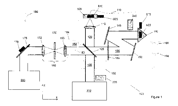
Referring now to Figures 1 to 3, an example implementation of an OCT
system is illustrated comprising three main sections. The first section, shown
in
Figure 1, is the main interferometer body 100, which splits and recombines the
light and allows interference to occur. The second section, shown in Figure 2,
is
the sample scanning system 200. This system takes the light from the sample
arm of the interferometer and directs it onto the sample under observation
(typically using via a scanning operation), allowing for a 3D reconstruction
of the
sample structure. The third section, referred to below as the backend 300, is
shown in Figure 3 and comprises a spectrometer that disperses the light from
the
interferometer and acquires the spectral interference data.
The light from the optical source 105 (shown as a fiber launcher for
emitting light from a fiber coupled semiconductor laser diode) enters system
100
through a single mode fiber 110 matched to the laser diode. The FC-APC coupler
on this fiber 110 is designed to minimize back reflections into the laser
diode 105,
which can damage the device. This fiber has a numerical aperture (NA) of 0.14
12
CA 02817104 2013-05-06
WO 2012/065267 PCT/CA2011/050710
and is collimated by a near-infrared achromatic lens 115 (Thorlabs AC254-75-B
f
= 75 mm) to provide a collimated beam (with a diameter of 21 mm). The
collimated beam 120 is then sent into the main interferometer body.
Inside the interferometer, the collimated beam 120 is split using a beam
splitter 125 (Thorlabs BSW17 non-polarizing 2" plate) and the two collimated
beams 130, 135 are directed to the sample system and the reference arm,
respectively. The reference arm primarily consists of a retroreflector 140
(CV!
MeIles Griot CCH-25.4-1-LEBG 1" hollow retroreflector), several beam steering
mirrors 145, 150 (Thorlabs PF20-03-P01) to compress the beam path, and a
neutral density filter 155 to reduce the reference intensity. The light from
the
reference arm is reflected from the retroreflector 140 and returns to the beam
splitter 125 for recombination.
Referring now to Figure 2, the sample scanning system includes a
galvanometer scanning mirror system 205 (Nutfield QuantumScan-30 1"
galvanometer), a sample focusing lens 210 (Thorlabs AC508-100-B 100 mm 2"
NIR achromatic), and a motorized translation stage 215 (Nanomotion FB050 50
mm stage) attached to angle bracket 218. A pair of mirrors 220, 225 is
employed
to dogleg the beam and direct it to the galvanometer 205, which is provided to
enable lateral scanning of the beam across the sample 230 (preferably with
micron level resolution) by changing the angle of incidence on the sample
focusing lens 210. The light reflecting off the galvanometer 205 enters the
sample focusing lens 210 and is focused onto a sample platform mounted on the
translation stage 215. The translation stage 215 enables the positioning of
the
13
CA 02817104 2013-05-06
WO 2012/065267 PCT/CA2011/050710
sample 230 in a direction orthogonal to the galvanometer scan direction (the
Nanomotion translation stage employed in the example system provides 10 nm
resolution and 50 nm repeatability). Together, the translation stage 215 and
galvanometer 205 support scanning the beam across the sample 230, with the
An additional translation stage (not shown; New Focus 9064-X) provides
sample focus adjustment ( 14 mm using the equipment quoted). The beam
incident on the sample 230 scatters back into the sample focusing lens 210 and
returns to the beam splitter 125 for recombination.
When the light from both arms returns to the beam splitter 125, half the
light is returned towards optical fiber 110 (and lost) while the other half is
sent to
a spatial filter system 160. The spatial filter system 160 comprises a lens
165
(with a Thorlabs AC254-75-B 75 mm NIR achromatic) which focuses the
collimated beam onto a pinhole 170 (Newport 910-PH10 10 pm). Pinhole 170
Referring to Figure 3, in spectrometer backend 300, a grating 305 is
provided to spectrally and spatially disperse the transmitted light. In the
example
experimental system used, the grating selected was a custom Kaiser Optical
grating with 1,200 lines per mm (I/mm), and was designed to maximize the
14
CA 02817104 2013-05-06
WO 2012/065267 PCT/CA2011/050710
spectral throughput from the laser diode light source. The collimated beam 310
passes through the grating and the dispersed light 315 is focused by a lens
320
(Thorlabs AC508-150-B 150 mm NIR achromatic). The focused light is directed
onto and detected by a line scan camera 325 (Basler Sprint spL2048-70km) and
interfaced with a personal computer using an image acquisition board (not
shown; National Instruments NI PCIe-1429 Camera Link).
In a system involving a fiber optic based design, most of the alignment is
handled by the high precision couplers attached to the fiber optic components.
This makes for simple assembly and a robust implementation but requires the
use of fiber optics in the interferometer. In the present free space system
shown
in Figures 1-3, the alignment of the OCT system will drift if not controlled.
The
following description addresses the design of an automatic alignment system
for
maintaining the stability of the interferometric system.
To obtain interferometric fringes on the line scan detector, it is important
for spatial coherence to be achieved and maintained at the detector. It is
also
important to ensure that the light paths continue to propagate through the
system
in the presence of alignment perturbations. In the present frequency domain
(FD)-OCT based design, the temporal coherence constraints are limited by the
bandwidth of a pixel in the backend spectrometer 300 rather than by the
bandwidth of the light source. In this case, optimal use of a 2048 pixel
detector
with a 100 nm bandpass would provide a pixel bandwidth of approximately 0.05
nm. The laser diode light source has a central wavelength of 850 nm, providing
a
coherence length of about 15 mm. Maintaining the beams within such a
CA 02817104 2013-05-06
WO 2012/065267 PCT/CA2011/050710
coherence length is readily achievable. Even with bandwidths many times this
optimal value, millimeter level offsets are generally acceptable.
The spatial coherence constraints of the system are determined by the
angular size of the source emitted from the fiber launcher 105 and the pinhole
170. Both of these are on the order of 10 pm with a 75 mm focal length
focusing
lens 165. This yields a coherence area of about 45 mm2 for the shortest
wavelengths of the source. This corresponds to a circular region with a
diameter
of approximately 7.5 mm. This is about one third of the beam diameter and is
also readily achieved.
Although maintaining coherence is readily achievable, small tilt errors can
greatly offset the position of the spots in the system. Assuming 10 pm spots
are
obtained with a 75 mm focal length lens 165, an induced tilt of 30 arcseconds
would be sufficient to offset the focus by an entire spot width. Such a 30
arcsecond tilt would be induced by about a 2 pm skew in a 1" diameter optic
(and
even less in some optics). A small fraction of this distance is sufficient to
significantly affect the system performance. Such small errors are likely to
occur
and it is important to provide a feedback mechanism for their correction.
The timescales for relative system alignment are estimated as follows. A
typical lens mount (such as a Thorlabs LMR1) has an aluminum base height of
about 10 mm. The coefficient of thermal expansion of aluminum is about 23
x10-6 m/m C near room temperature. A 1 C temperature change would induce a
shift of 0.2 pm in this mount. When the combined effect of many such mounts
and the hardware required to affix these mounts in the system is considered, a
16
CA 02817104 2013-05-06
WO 2012/065267
PCT/CA2011/050710
temperature changes on the order of 1 C can have a relatively large effect on
the
efficiency of the system. Without thermal isolation, a person's body heat near
the
system could be enough to disrupt alignment. Without significant thermal
isolation, alignment will drift as the system temperature changes.
Because all the components in the system are attached typically to a fixed
substrate (such as an optical bench or breadboard), a small amount of
vibrational
isolation should result in most of the misalignment sources arising from
temperature variations. Because it is expected that the system is to be used
indoors, it is likely that the temperature variations will occur on long
timescales.
For example, in the laboratory environment in which the present system was
built, it was possible to use the system with people in the room for several
hours
without significant image degradation. Nonetheless, alignment was found to
improve system throughput, especially when performed before beginning any
data collection.
Due to the nature of OCT imaging, several mitigating factors reduce the
tolerances placed on the alignment system. First, the light from the sample
returns with a much larger effective spot than the specular reflection off a
mirror
surface (see Figure 4). While some of this is multiply scattered light, the
majority
of the signal near the center of this spot is useful singly scattered light.
Although
it is desirable to isolate a small portion of this light to focus on a
specific lateral
point in the sample, a small misalignment will primarily shift the point of
interest
rather than significantly reducing the returned signal.
On a similar note, the light in the reference arm generally needs to be
17
CA 02817104 2013-05-06
WO 2012/065267 PCT/CA2011/050710
significantly reduced (for example, using one or more neutral density (ND)
filters)
to provide an appropriate signal level to mix with the sample light. The
primary
result of a misalignment in the reference arm is a reduction in signal
strength,
with a secondary spectral shift due to an imperfectly achromatic lens. The
signal
strength reduction is readily compensated by a change in ND value and
experiment calibration data can be employed to mitigate the spectral shift
effect.
These two effects, when combined, limit the effects of instantaneous
system misalignment, with the result that the more stringent requirements
relate
to the long term stability of the system.
The inventors have found that the important degrees of freedom for
alignment of an optical interferometric system can be significantly reduced by
assessing the relative contribution of each apparent degree of freedom to
misalignment. Each component in an optical system has 6 degrees of freedom:
translation and rotation axes for the x, y, and z dimensions. Aligning every
possible axis of the components in a complex system is unfeasible ¨ for
example, well over 50 axes of control would be needed to accomplish this task.
One aspect of the present auto-alignment systems and methods is the reduction
of the required control axes. This may be achieved by identifying insensitive
degrees of freedom and combining complementary degrees of freedom into a
smaller number of controls. It is generally assumed that the errors to be
corrected are reasonably small, such as those caused by moderate temperature
fluctuations or by small shocks to the system.
The identification and reduction of the relevant degrees of freedom can be
18
CA 02817104 2013-05-06
WO 2012/065267 PCT/CA2011/050710
performed as follows. First, the degrees of freedom that cause a noticeable
effect
for the various types of components are identified. As an example, each of the
optical components is rotationally symmetric, immediately removing one degree
of rotational freedom from consideration. Table 1 enumerates the effect of the
various degrees of freedom on the optical components. This table makes
assumptions based on the design ¨ for example, that all of the main OCT system
mirrors operate on collimated light.
Degree of Fiber Pinhole Lens Mirror Retroreflector
Freedom Launcher
Translation X Tilt Tilt Tilt ¨ Shear
Translation Y Tilt Tilt Tilt ¨ Shear
Translation Z Focus Focus Focus Shear and Path Length
Path Length
Rotation X Shear ¨ Focus Tilt ¨
Rotation Y Shear ¨ Focus Tilt ¨
Rotation Z ¨ ¨ ¨ ¨ ¨
Table 1: The effect of degrees of freedom of the various optical components on
the optical alignment of the system. The degrees of freedom are referenced to
the centers of the optical components.
With small errors, the optical effects in the system may compound. As an
example, if a mirror is expected to induce tilt, then the mirror tilt will be
added to
any original beam tilt. As long as the errors remain small, this error may be
corrected in the system by adjusting a single component with the opposite
effect.
This principle allows for the simplification of the correction protocol.
Accordingly, the reduction of the degrees of freedom of the system
involves determining how the relevant degrees of freedom will affect the
system
alignment and performance. For simplicity, in the context of the present
example,
this is described by analyzing the system in terms of five smaller subsystems:
19
CA 02817104 2013-05-06
WO 2012/065267 PCT/CA2011/050710
fiber collimation, the reference arm, the sample arm, recombination, and the
spectrometer.
Fiber collimation primarily consists of the fiber launcher (shown generally
at 105) and a collimating lens 115. From Table 1, it is evident that the
important
effects to consider are focus, shear, and tilt. The depth of field of the
collimation
lens is large enough that most focus misalignments have a negligible effect on
the system ¨ as an example, the thermal expansion of aluminum gives provides
a 15 C window before the depth of field is exceeded in the present example. In
addition, the focus of the sample arm compensates for a defocus entering the
sample arm and an adjustment of attenuation of the neutral density filter 155
in
the reference arm can compensate for lost light passing through the pinhole.
Any
shear introduced at this point will be small relative to the pupil diameter
and will
affect both arms of the interferometer equally, making any effect small. Tilts
introduced here are very significant, though, with degree level temperature
fluctuations shifting the spot location by large fractions of the spot size.
Accordingly, because of the sensitivity of the fiber launcher 105 to tilt,
tilt
corrections are provided at the fiber launcher. Implementing system tilt
control is
possible by moving the position of the input fiber relative to the collimating
lens.
The tilt corrections are achieved by providing a pair of motorized horizontal
605
and vertical 610 translation stages, which, through the translation of the
fiber
launcher relative to the collimation lens 115, facilitate tilt correction of
the source
beam. In the example system shown in Figures 1-3, a New Focus 8051 pico fiber
launcher 105 was employed for positioning the fiber with 30 nm step sizes over
a
CA 02817104 2013-05-06
WO 2012/065267 PCT/CA2011/050710
3 mm range. With the 75 mm collimating lens 115, this allows for tilt
adjustments of approximately 80 milliarcseconds over a 2 range. This degree
of tilt control is sufficient to maintain alignment at a high level. By
manipulating
the tilt through the fiber launcher using the motorized translation stages 605
and
610, the dominant residual misalignment may be corrected so that the beams
pass the OCT signal through the pinhole and into the spectrometer backend.
Turning now to the reference arm, the light partially reflects off the beam
splitter 125 and a pair of fold mirrors (150, 145) and then encounters the
retroreflector 140. Because of the design of the retroreflector, light
entering the
retroreflector is reflected with the same tilt (with less than one arcsecond
error)
but offset in shear by double the original amount. The long path length in the
reference arm also converts any tilts into a small shear. By reflecting off of
the
fold mirrors 145 and 150 twice, any residual tilt effect is removed, but the
mirrors
can still induce additional shear. Overall, only the tilt induced by the beam
splitter
125 will affect the tilt of the reference arm output.
To overcome the shear that can be induced in the reference arm,
motorized shear control is integrated to the retroreflector 140 to enable
shear
correction. This correction enables control of the overlap of the reference
135
and sample 130 beams. The shear corrections are achieved by providing a pair
of motorized horizontal 615 and vertical 620 translation stages, which, via
translation of the retroreflector 140, enable shear compensation in the
reference
arm. In the case of the present example, mounting the retroreflector on two
orthogonal translation stages (New Focus 9067-COM) with two attached New
21
CA 02817104 2013-05-06
WO 2012/065267 PCT/CA2011/050710
Focus 8302 picomotors allows for shear adjustment of the returning reference
beam. The New Focus 8302 picomotors provide for 0.5" of translation with 30
nm step sizes, allowing the system to maintain coincidence at a small fraction
of
the beam diameter.
Regarding the sample arm, the collimated beam 130 entering subsystem
200 (shown in Figure 2) reflects off mirrors 225 and 220 and is then focused
onto
the sample via lens 210. In the case of OCT, the primary performance concern
relates to the light that back reflects from the sample in a single scattering
process. This is light that is reflected back the same way it enters, which
ensures
that light entering the sample arm returns along the same path it enters.
Therefore any alignment errors in the sample arm correct for themselves as the
light travels back along the path it enters. The light then reflects off of
the beam
splitter 125 and gains the same tilt induced before light entered the
reference
arm.
After passing through the reference and sample arms, the light beams are
recombined through and focused through the spatial filter pinhole. At this
point in
the system, the following misalignments may exist: an initial tilt and shear
introduced by the fiber collimation, tilt induced by the beam splitter 125,
and
shear induced by the reference arm. The shear in the reference arm can be
corrected through motorized shear control in the reference arm, as noted
above.
This leaves a tilt and small shear that may exist in the beam. The residual
shear
will be a small fraction of the collimated beam diameter and should cause
little
issue. The tilt will determine the spot location and it is important to ensure
that
22
CA 02817104 2013-05-06
WO 2012/065267 PCT/CA2011/050710
the spot location and pinhole location coincide.
It was found by the inventors that frequent alignment of the spectrometer
is not generally required ¨ adjustment of the spectrometer was not found to be
needed over a timescale of many months despite performing tilt and shear
correction in the interferometer. Temperature testing, however, revealed a
need
for alignment with large temperature changes, and such alignment primarily
involved vertical position on the focal plane, which can be adjusted by
tilting one
axis of the fold mirror 175. Because of the small vertical height of the
detector,
this is the most sensitive degree of freedom in the spectrometer. Horizontal
positioning is relatively insensitive due to the large focal plane width
(assuming
spectrometer calibration is performed), the depth of field is sufficiently
large that
focal effects are minimal, and any shear induced will also be minimal.
Accordingly, for environments with in which large temperature fluctuations
are expected, an additional axis of control may be provided on the fold mirror
feeding the spectrometer, as noted above. A single motor 178 (e.g. a
Picomotor)
attached to the vertical axis of a mirror mount (e.g. Thorlabs KM200 kinematic
2")
provides the control flexibility for this axis. With the goal of maintaining
light on a
detector with large system variations, feedback may be provided by simply
employing the final system detector to correct for offsets in this axis.
Despite all the potential locations for misalignments in the system, the
preceding analysis suggests that two axes of tilt control and two axes of
shear
control are sufficient to adequately maintain system alignment. With large
temperature variations (larger than those seen in the laboratory environment
23
CA 02817104 2013-05-06
WO 2012/065267 PCT/CA2011/050710
under normal conditions), an additional axis is required to control the
vertical
position of the beam incident on the spectrometer.
In order to maintain system alignment, additional hardware providing
feedback to monitor and adjust the alignment is required. To minimize the cost
and complexity, the number of alignment components should be minimized. This
involves identifying the unique degrees of freedom in the system and providing
monitoring and control devices for them.
The preceding examination of the system shows that two degrees of
alignment freedom should be sufficient to monitor and maintain interferometer
alignment. As noted above, alignment can be maintained by adjusting the tilt
of
the beam entering the interferometer to ensure the spots in the system pass
through the pinhole. In addition, the retroreflector position can be adjusted
to
ensure that the two interferometer arm beams are coincident. By monitoring and
controlling these four degrees of freedom (vertical and horizontal tilt and
shear), it
is possible to correct for the dominant system drifts. By aligning the system
at the
pinhole, it can be ensured that a clean interferometric signal enters the
backend
with both the reference and sample beams coincident.
In addition to adjusting the system alignment, it is important to measure
the deviation from proper alignment and determine the required corrections
according to a feedback scheme. Ideally, the system should be able to monitor
alignment at all times while being minimally invasive. Because it is expected
that
the alignment drifts will occur over a long time frame relative to the
acquisition
rate of the system, a small fraction of the light from the system may be split
off to
24
CA 02817104 2013-05-06
WO 2012/065267 PCT/CA2011/050710
monitor the system alignment. For example, a 0.2% anti-reflection (AR) coated
beam sampler 180 may be employed to maintain a sufficient frame rate for an
alignment measurement system while maintaining the very high system
throughput.
In order to monitor the presence of a tilt offset, a reflective pinhole is
employed and a reimaging system is implemented. Placing the beam sampler
180 before the pinhole focusing lens 165 but after the beam splitter 125 sends
an
image of the pinhole plane out of the beam path of the interferometer as
collimated beam 182. By focusing this light with lens 184 (Thorlabs AC254-300-
B
300 mm focal length achromatic) onto an imaging detector 186 (IDS model Ul-
1225LE-M) an image of the pinhole is obtained (in the present case, the
pinhole
image is provided with a 7 pixel diameter). This allows for the measurement of
tilt
offset at the sub arcsecond level. Adjusting the focal length of this imaging
system allows one to trade off measurement accuracy for measurement speed.
Because the beam sampler reflects the light reflecting off the pinhole and
the light entering the spatial filter system in opposite directions, the same
beam
sampler may also be employed to image the pupil offset of the reference and
sample beams. Imaging these beams through a beam reducer (comprising
lenses 192 and 194) with another imaging detector 196 allows us to measure the
coincidence of the sample and reference collimated beams 130 and 135. By
adjusting the parameters of the beam reducer, the imaging speed versus the
measurement accuracy can be optimized.
One of the important features of the system is the ability to determine
CA 02817104 2013-05-06
WO 2012/065267 PCT/CA2011/050710
alignment errors and to automatically correct for these errors. Errors will be
manifested as offsets from the expected positions of the beams on the
alignment
cameras. By quantifying these offsets using a feedback scheme, the system can
automatically determine the corrections that are needed to improve the system
alignment.
Figures 5 and 6 show the ability of the system to detect alignment offsets
and the effect the offsets have on the final interferometric and spectrally
resolved
signal. Figure 5 shows various levels of tilt offset detected by the tilt
monitoring
system described in the examples provided herein. As the tilt offset increases
(increased distance between the tilt measurement crosshairs), less light is
transmitted through the pinhole. By moving the tilt controls to place the
offset
spot back on the alignment crosshairs, the lost signal can be recovered.
Figure 6
shows various levels of detected shear offset by the shear monitoring system.
A
crosshair with a small line indicates the direction and magnitude of the
offset
corresponding to the signal losses detected in the lower images. By correcting
the offset, it is possible to recover the lost signal and return to the
original signal
strength.
The system tilt is manifested as a positional offset of the focused spot on
the pinhole plane. An offset of this spot from the pinhole produces two main
effects: the centroid of the reflected light off the pinhole plane shifts and
the
intensity of the reflected light increases (due to less light passing through
the
pinhole). The goal of the automatic alignment system is to determine the
correction to compensate for any tilt offset induced in the beam.
26
CA 02817104 2013-05-06
WO 2012/065267 PCT/CA2011/050710
If a perfectly focused spot from the fiber input is reimaging on the pinhole,
it will resemble an Airy disk, the diffraction pattern caused by the finite
aperture
optics. It will have a very bright core (which is the signal to be passed
through the
pinhole under an aligned state) along with much dimmer rings. If further
imperfections from a diffraction limited spot occur, they will pull light from
the core
into the wings ¨ and such light outside the core is the light that is to be
blocked
with the pinhole.
The core of the Airy pattern contains approximately 84% of the total
intensity, with the first ring containing approximately 7% and the second ring
containing approximately 3%. Accordingly, even in the ideal case, a
significant
fraction of the incident light will be reflected by the reflective portion of
the pinhole
mount and provide useful a signal for alignment monitoring. Despite this, the
required dynamic range for monitoring the entire Airy pattern is large¨the
peak
intensity of the first ring is less than 2% of the peak intensity of the
central core.
The equipment employed in the present example provided included a detector
with only 8 bits of discrimination (256 levels), with the consequence that
obtaining sufficient contrast on the rings will cause saturation in the core
if the
beam core fails to pass through the pinhole.
Assuming the system begins in an aligned state, it is desirable to maintain
the position of the focused spot on the pinhole plane. It is important to be
able to
identify the desired position and maintain such a position. To achieve this,
an
appropriate direction and magnitude of corrective motion for any offset should
be
determined. With a fixed sample in the system, the pattern of light on the
pinhole
27
CA 02817104 2013-05-06
WO 2012/065267 PCT/CA2011/050710
plane stays constant. Changing the tilt of the system shifts this pattern in a
deterministic direction. The centroid of this pattern provides an indicator of
the
offset from the desired position.
In calculating the centroid, many different methods can be employed. Two
example methods are provided below. When a bright and clean spot illuminates
the pinhole (such as with the reflection off a mirror in the sample arm, see
Figure
4(a)), weighting the centroid by the intensity of the pixel value enhances the
accuracy by accounting for the brighter center of the spot. However, when a
more irregular sample is placed in the sample arm (providing a reimaged spot
similar to that in Figure 4(d)), intensity weighting can greatly skew the
centroid
location. It has been found that simply thresholding the image and centroiding
the
thresholded pixels without weighting provides a superior response in this case
¨
and the reduced information per pixel is believed to be offset by a larger
number
of illuminated pixels.
Despite the potential for saturation when the core is not optimally incident
on the pinhole, the exposure time can be set to properly image the position
when
the light passes through the pinhole. It has been found that the 8 bit imaging
camera employed in the experimental testing of the system still operates well
when saturated by the core, allowing sufficiently accurate measurements to
move the core into the pinhole according to an automatic alignment protocol.
As
the core moves into the pinhole, the light diminishes and eliminates the
saturation, and it is still possible to measure the correct offset. If the
exposure
time is set to properly image the core, the signal will be too dim for proper
28
CA 02817104 2013-05-06
WO 2012/065267
PCT/CA2011/050710
measurement when the core enters the pinhole. In another embodiment, an
adaptive exposure time method could be employed to provide improved dynamic
range, where the exposure time is determined by the pixel intensity and is
selected to avoid saturation.
The shear offset measurement system images the collimated beams in
the interferometric system. The shear offset system is employed to ensure that
both beams in the system pass through the system together and pass through
the focusing lens be imaged onto the pinhole.
Identifying the two separate beams can be easily (but invasively)
performed by using beam blockers (Figure 1 shows beam blockers 335 and 340
that can be inserted into the collimated beam paths 130 and 135,
respectively).
Fortunately, the two pupils do not change significantly with small shears. By
storing the individual pupil images, it is possible to compare shifted
summations
to a combined image to extract the position of each pupil, without blocking
each
individual beam and halting the overall system. The required shift to generate
the
combined image provides the offset of the pupil from the original position.
In one embodiment, an alignment correction algorithm involves assuming
that an initial satisfactory alignment state is known and maintaining that
alignment state under feedback. While such an algorithm will be useful when
the
system is operated from an initially aligned state (such as when the system is
first assembled), the interferometric system will naturally undergo
misalignments
and it is useful to also provide a method of determining a suitable initial
alignment
position.
29
CA 02817104 2013-05-06
WO 2012/065267 PCT/CA2011/050710
As the present embodiment is primarily concerned with obtaining a
suitable signal from the final detector, this detector can be used (at least
in part)
as a source of feedback information to assess the system alignment. One
limitation is that the alignment must already provide sufficient light to this
detector
¨ the light must already be at least partially passing through the pinhole.
The
large field of view of the alignment cameras allows us to sufficiently align
the
system for signal to reach the final camera even if corrections are needed for
better alignment. Once a signal is obtained on the final detector, this signal
can
be employed to improve the alignment and calibrate out any accrued alignment
system errors.
In one embodiment, the initial alignment method is achieved as follows. By
focusing on a mirror in the sample arm, a focused spot resembling an Airy
pattern is obtained, characterized by a very bright core with a fading
intensity
farther from the center (see Figure 4(a)). By blocking the reference arm with
the
beam blocker 340 and adjusting the tilt motors 605 and 610, it is possible to
adjust the amount of light returning from the sample arm mirror that passes
through the pinhole, where this adjustment is made without interference
effects
caused by the reference arm. Because the spot core possesses a smooth profile,
a simple gradient following algorithm with reducing step sizes is sufficient
to
maximize the sample signal. This measurement can be performed by the final
system camera (325), ensuring that we maximize the signal detected by the
final
system and not rely entirely on the alignment system for calibration.
Once the sample arm is aligned, the shear control may be adjusted to
CA 02817104 2013-05-06
WO 2012/065267 PCT/CA2011/050710
align the reference arm. To avoid interference effects affecting the measured
signal, the sample arm is blocked using beam block 335. Again, a simple
gradient following algorithm with reducing step sizes is sufficient to
maximize the
reference signal. In one embodiment, the beam blocks 335 and 340 are
motorized, enabling automated insertion of the beam blocks into the respective
beam paths, thus enabling full automation of the present initial alignment
procedure.
In a similar fashion, the vertical position of the light hitting the
spectrometer may be adjusted. As this control affects both arms equally, the
signal from both arms may be employed to maximize the total throughput. The
interference between the two arms should be substantially constant at this
point,
and therefore the blocking of individual arms is typically not necessary.
After having obtained an initial alignment state, the alignment method
according to one embodiment monitors changes from the initial state and
corrects for alignment errors using the alignment feedback and controls. In
one
embodiment, when the system is properly aligned, the system state is recorded,
for example, in a series of variables, where the recorded system state enables
the determination of offsets from this state. Even with large system changes
(for
example, including alignment offsets that render the system completely
unusable), the recorded offsets allow for the system to be quickly returned to
a
state that is close to the previously aligned state.
In one embodiment, the automated alignment system determines the
initial alignment state by accessing primary system components (such as the
31
CA 02817104 2013-05-06
WO 2012/065267 PCT/CA2011/050710
final OCT detector) to accurately determine a suitable alignment state with
desired performance. This optimization is an intrusive process and it may
place
limitations on the range of parameter space in which the system may reside
prior
to the automated determination of the initial alignment state. Moreover, due
to its
intrusive nature, such a method is not suitable for constant system
monitoring,
but provides a suitable initial state and can correct for errors accruing in
the
alignment system. Combined with the primary automated alignment scheme, the
overall system and method are generally able to maintain high quality short
and
long term system alignment.
During operation of the alignment method, alignment offsets from an initial
state are determined. Given the calculated offsets, the errors are corrected
by
moving the various alignment motors 605, 610, 615 and 620 to translate the
input
source and retroreflector for the correction of tilt and shear, respectively.
However, in order to determine the appropriate corrections, it is important to
calibrate the alignment system in order to obtain the relationship between
camera offsets and motor movements.
Such a calibration may be performed manually or in an automated
fashion, with the resulting calibration parameters stored and accessible by
the
computing system that is employed to automate the alignment method. In one
embodiment, the calibration is performed automatically by the alignment
software
interface, although this requires the operation of the system to be suspended.
By
moving each axis of the system individually by a known amount and computing
the apparent movement, it is possible to determine the effect each axis has on
32
CA 02817104 2013-05-06
WO 2012/065267 PCT/CA2011/050710
the system and thus calibrate the system. It is important to note that the
mount
loading forces may cause forward and reverse motor movement commands to
react differently (e.g. due to motor backlash), which may require a different
calibration procedure for each direction. The calibration may be stored in a
multitude of different formats, including, but not limited to, a look-up table
(for
interpolation) and a mathematically fitted relationship.
The motor calibration data and the measured offsets are then employed to
determine an appropriate motor response (e.g. motor commands, steps, and/or
drive voltages and time intervals) to improve the current system alignment. By
iteratively measuring the offset and correcting the offset, a feedback loop
may be
employed to maintain alignment. In one embodiment, damping (for example,
reducing the commanded positions by a fixed factor, such as 25%, to slow the
convergence and prevent overshooting) is provided to compensate for small
errors or drifts in the motor calibration (with an increased response time).
With reference to Figure 7, a flow chart 400 is provided that illustrates the
steps involved in the automated alignment method disclosed above. In step 405,
the interferometric system is constructed and aligned. The initial alignment
state
is stored in step 410 based on the positions of the spot and beam centroids in
the
tilt and shear imaging cameras, respectively. The system is then operated, and
after a given time interval, the alignment of the system is assessed. In step
415,
the tilt offset is calculated based on the deviation of the spot centroid as
measured using the tilt imaging camera. Using the appropriate calibration
data,
the tilt correction system is activated in step 420 to correct for the tilt
offset. In
33
CA 02817104 2013-05-06
WO 2012/065267 PCT/CA2011/050710
step 425, the shear offset is calculated based on the observed beam shear in
the
shear imaging camera. The calculated shear offset and appropriate calibration
data are then employed in step 430 to correct the observed shear. While steps
415 and 420 are shown as occurring prior to steps 425 and 430, it is to be
understood that the order of performing these pairs of steps may be reversed.
After having performed the tilt and shear corrections, a determination is
made in step 440 as to whether or not an overall system calibration should be
performed. As noted above, such a determination can be made based on a
measured signal indicative of the system performance, such as the signal
obtained at the spectrometer. This determination can be made by examining the
throughput from a well calibrated sample, examining the reference arm
intensity
compared to a previously calibrated amount, or other methods to determine a
decrease in system sensitivity. The shear and tilt are then optimized in steps
445
through 455, which may be performed by blocking the individual interferometer
beams serially and optimizing each beam separately. If sufficient convergence
has been obtained in step 460, the current alignment state is stored once
again
in step 410, and the tilt and shear offset correction portion of the method is
repeated. If convergence has not been reached, steps 445-455 are repeated.
In one embodiment, the alignment feedback loop may be configured to
pause prior to performing a given alignment correction in order to obtain
human
verification. Using a user interface that is interfaced with the computing
system
performing the automated alignment method, a human controller may verify that
a calculated correction is reasonable before allowing the system to implement
34
CA 02817104 2013-05-06
WO 2012/065267 PCT/CA2011/050710
the correction. By repeating this process for both tilt and shear, the system
is
able to recover and maintain system alignment. In another embodiment,
corrections are automatically performed without requiring human input for
verification.
Although the preceding embodiments were described in the context of an
example implementation of a system with specific examples of system
components and performance figures, it is to be understood that the
embodiments are not limited to the examples provided. A wide variety of system
configurations and components may be employed without departing from the
scope of the claimed embodiments. For example, the OCT system may involve a
time-domain interferometer as opposed to a frequency domain interferometer. In
another variation, the optical source may comprise direct emission from a
laser,
where the relative position of the laser is controlled for tilt alignment
using motors
605 and 610.
It is important to recognize that the system is not limited to OCT system
applications, and may instead be adapted to provide systems and methods for
the automatic alignment of a wide variety of interferometric optical systems.
Generally speaking, by isolating the necessary degrees of freedom and
implementing measurement and correction hardware, an alignment system can
be implemented according to the embodiments disclosed herein.
As described above in relation to the OCT example, the first objective in
the design process is the identification of the dominant degrees of freedom in
a
given interferometric system. Such dominant degrees of freedom are the degrees
CA 02817104 2013-05-06
WO 2012/065267 PCT/CA2011/050710
of freedom that have a substantial effect on system performance if alignment
changes occur. Although the dominant degrees of freedom depend on the actual
system configuration employed, general guidelines for the identification of
the
dominant degrees of freedom are provided in the following description.
Firstly, it is important to determine the characteristics of the light
interacting with each optic. If the light is converging, diverging,
collimated, or a
focused spot, different effects will result from different components. In the
example OCT system, the beams were typically focused or collimated light.
The effect each individual component will have on the light path is then
determined. Light incident on a flat mirror, a lens, a curved mirror, or other
optical
surfaces will all behave differently. The initial characteristics of the light
at that
surface will also matter. For systems characterized primarily by simple
surfaces
(such as flat mirrors, circularly symmetric lenses operating on collimated
light,
and similar), a geometric analysis is typically sufficient. When more complex
optics are used, it may be important to model the beam propagation using
simulation software such as ZEMAX (especially if the effect of one optic is
expected to cause significant changes to the operation of another optic). Some
specific examples are briefly provided in the forthcoming paragraphs.
A flat mirror operating on collimated light is one of the simpler optics to
consider. Light reflecting off a flat mirror is reflected about the normal of
the
mirror surface. For collimated light, all the beams are travelling in the same
direction and produce the same reflection. Four degrees of freedom (rotation
about the normal, translation in two orthogonal dimensions perpendicular to
the
36
CA 02817104 2013-05-06
WO 2012/065267 PCT/CA2011/050710
normal, and translation along the normal) have no effect on the direction of
the
normal¨movement in these directions will not affect the reflection angle.
The two remaining degrees of freedom cause a rotation of the normal,
which leads to a different reflection angle of the beams. In addition,
translation
along the normal, while not affecting the direction of reflection, will change
the
incident point, potentially changing the path length and shear of the beam.
With
large movements, it is also possible for any degree of freedom other than
rotation
about the normal to cause the incident light to bypass the mirror. These
effects
are illustrated in Figure 8.
A standard lens converts a collimated beam into a focused spot over a
specific focal length and vice versa. In the ideal case, tilts in the
collimated beam
are converted to positional shifts in the focal plane while shears simply tilt
the
cone angle. In reverse, a positional shift in the focused spot causes a tilt
in the
collimated beam while the incoming angle of the light from the spot determines
the location of collimated beam (i.e., its shear).
If the lens rotates about the optical axis, nothing changes. If the lens
shears along the optical axis, the focal point of the lens shifts. If it
shears
perpendicular to this axis, the effect will vary depending on the direction of
light
propagation¨if the lens is collimating light then a tilt will be seen in the
collimated beam, while if the lens is focusing collimated light then the light
will
focus to a different point. If the lens tilts, this will rotate the focal
plane and
change the focused light position. As with the mirror, large enough shifts or
rotations can cause the beam to completely miss the lens but this is an
extreme
37
CA 02817104 2013-05-06
WO 2012/065267 PCT/CA2011/050710
case. These effects are illustrated in Figure 9.
A single mode fiber can be approximated as a point source emitting light
in a specified cone. If this light is to be collimated by a lens, the effects
are
related to those caused by a lens. If the position of the fiber changes on the
focal
plane of the lens, a tilt will be generated in the collimated beam leaving the
lens.
If the exit of the fiber leaves the focal plane of the lens, a defocus is
caused. If
the exit cone of light from the fiber tilts, shear will be generated in the
collimated
beam.
A corner-cube retroreflector consists of three reflective surfaces forming a
shape similar to the corner of a room where ceiling or floor meets two side
walls.
This optical layout has several beneficial properties, a primary one being
strong
tilt insensitivity¨a beam entering the retroreflector exits with the same tilt
as the
incoming beam, as if bouncing off a flat mirror with a normal closely aligned
to
the optical axis. Unlike a flat mirror, though, any beam shear (or,
equivalently, a
shear in the retroreflector) is flipped about the center of the
retroreflector. This
effect has both advantages and disadvantages¨while the sensitivity to shear
can cause beam position errors, it can also be used to accurately cause an
offset
in beam position with no change in tilt.
Similar analyses can be performed for other optical components. After
identifying all the possible degrees of freedom, they can be reduced to
identify
those that have a net effect of the system, and an alignment controls can be
provided for the reduced set of dominant degree of freedom. This process is
discussed in further depth below.
38
CA 02817104 2013-05-06
WO 2012/065267
PCT/CA2011/050710
After having identified the effect of errors in each optical component, the
next step in the method is the determination of the required controls to
correct for
these errors. First, the dominant degrees of freedom are isolated as those
that
produce misalignment errors that have a substantial and/or important impact on
system performance. Misalignments may generate problems due to beam or tilt
offsets at the final detector (where an error changes the detected signal) or
at an
intermediate location such as a pinhole plane (where an error can cause the
light
to no longer propagate through the system). Such locations correspond to
positions at which the system alignment is to be monitored in order to provide
feedback for the correction of errors. It is also important to identify which
optical
components and/or subsystems contribute to detectable errors at each relevant
location. These optical components are those at which corrections may need to
be performed to correct the errors.
After having identified where dominant errors can be corrected, the
dominant degrees of freedom that generate the errors are reduced (if possible)
into a smaller number of dominant degrees of freedom. For example, a tilt
caused by a mirror can be corrected by a tilt in the beam hitting the mirror.
This is
true even for multiple mirrors in series, allowing a single tilt correction to
handle
many different tilt contributions.
It is also important to note, at this point, that if the light returns along
the
same path it originally followed, many misalignments will be self-corrected.
This
can be seen, for example, by considering a beam that reflects off the same
mirror
twice from opposite directions¨when the beam first hits the mirror any error
term
39
CA 02817104 2013-05-06
WO 2012/065267 PCT/CA2011/050710
is added in but, on the return trip, the reverse error is added (effectively
subtracting out the original error). By identifying locations where this
occurs,
significant reduction in the number of required control surfaces can be
achieved.
Once all possible consolidations have been identified and a reduced set of
dominant degrees of freedom are obtained, one is left with a minimal number of
necessary correction axes. Monitoring and control apparatus may then be
implemented to measure and correct errors related to these axes. While the
implementation choice can vary for different systems, the apparatus and
algorithms similar to those described above for the OCT system are suitable
for
many different system configurations, and those skilled in the art will
appreciate
that the systems and methods can be readily extended to other interferometric
systems.
Referring now to Figure 10, a simplified example system is now provided
to illustrate the application of the preceding generic design methods, and to
provide a prescription of how the design method can be applied to other
interferometric systems.
Figure 10 shows an offset beam interferometer 500, which may be
employed in a Fourier Transform Spectrometer (FTS) or other interferometric
optical metrology system. The offset layout allows easy access to the
complementary outputs of the interferometer, collecting additional signal over
a
single output design. Collimated light enters the interferometer (in this
case,
collimating the output of a fiber 535 with a lens 540) and is split by beam
splitter
cube 505. The beam splitter cube 505 acts as a mirror for half the light
(sending
CA 02817104 2013-05-06
WO 2012/065267 PCT/CA2011/050710
light towards Retroreflector 510) and transmits the other half of the light.
Two
corner-cube retroreflectors (510 and 515) are employed to offset the beams and
return them to a second beam splitter cube 520. Half the light from
retroreflector
515 passes through the second beam splitter cube 520 and joins half the light
from retroreflector 510, which is reflected from beam splitter cube 520 to
form
collimated output beam 525.
The other half of light from retroreflector 515 reflects off beam splitter
cube
520 and joins with half the light from retroreflector 510 that is transmitting
through
beam splitting cube 520 to form collimated output beam 530. Complementary
interference effects due to phase shifts caused by different path lengths for
the
two arms of the interferometer provide the signals in outputs 525 and 530.
Examining the system according to the method outlined above, one notes
that there are six different optics that can have an effect on the alignment:
the
fiber 535, the collimating lens 540, the two beam splitter cubes 505 and 520,
and
the two retroreflectors 510 and 515.
Treating the beam splitter cubes 505 and 520 like mirrors for the reflective
path and ignoring them for the transmissive path, we can use the preceding
method to determine the effect of the various optical components on the
system.
In addition, one can readily identify the primary alignment points as being
located
at outputs 525 and 530.
Considering output 530, there is a focus effect from the fiber/collimating
lens pair 535 and 540, an overall tilt and shear from the same, a tilt in one
beam
from beam splitter cube 505 and a tilt in the other beam from beam splitter
cube
41
CA 02817104 2013-05-06
WO 2012/065267 PCT/CA2011/050710
520, and a shear in one beam from retroreflector 510 and in the other beam
from
retroreflector 515.
At output 525, there exists a focus effect from the fiber/collimating lens
pair 535 and 540, an overall tilt and shear from the same, a tilt in one beam
from
both beam splitter cubes 505 and 520, and a shear in one beam from
retroreflector 515 and in the other beam from retroreflector 510.
If an analysis of the consequences of the effects of misalignments on
system performance indicates that collimation is a significant factor, the
system
has only one place to affect the collimation, and corrections made here
propagate through the rest of the system equally. For the rest of the system,
it
may be important to account for the following: (1) that the two beams forming
output 530 have the same tilt, (2) the two beams at output 530 have the same
shear, (3) the two beams at output 525 have the same tilt, (4) the two beams
at
output 525 have the same shear, (5) outputs 525 and 530 have appropriate
overall tilts, and (6) outputs 525 and 530 have appropriate overall shears.
In order for criterion (1) to hold, beam splitter cube 505 and beam splitter
cube 520 should have the same tilt¨if this is not the case, the beams
reflecting
from beam splitter cube 505 and beam splitter cube 525 would each have a
different induced tilt after having started with the same tilt before entering
beam
splitter cube. The use of a single large beam splitter cube can mitigate this
effect,
although this can increase the amount of dispersive and absorptive glass in
the
system and does not allow for corrections of any imperfections in the
retroreflectors or splitting surface. Motorizing the tip and tilt of one beam
splitter
42
CA 02817104 2013-05-06
WO 2012/065267
PCT/CA2011/050710
cube provides the necessary alignment freedom to maintain this axis. A tilt
monitoring system (similar to the one used to monitor pinhole alignment in the
OCT system described above) can provide the necessary feedback for this axis.
For criterion (2) to hold, the beams should be coincident at beam splitter
cube 520 (if the two beams are coincident and have the same tilt, they will
stay
coincident as they travel further). Motorizing either of retroreflectors 510
and 515
can correct for any relative offset in the two beams and a shear monitoring
system similar to that in the OCT system disclosed above can measure this
offset.
It is noted that criterion (3) holds automatically if criterion (1) holds. The
beam that passes through both beam splitter cubes 505 and 520 (or one beam
splitter twice) accrues no tilt and the beam reflecting twice will cancel out
any tilt
on the second reflection. A similar relationship is true between criteria (2)
and (4)
¨ if the beams are coincident with the same tilt at the beam splitter, they
will
follow the same path leaving in both directions. This allows the same
components to be employed to ensure that both arms overlap in both outputs.
While it can now be ensured that both arms of the interferometer will be
overlapping at both outputs 525 and 530, the overall tilt (criterion 5) and
shear
(criterion 6) of these outputs may not be appropriate. Overall tilt can be
easily
added using the fiber position or collimating lens position, but these will
adjust
the two outputs simultaneously in opposite directions (because of the number
of
reflections seen by the two outputs). Also motorizing the tilt of the beam
splitters
allows for individual adjustment of the tilt of output 530 ¨ if output 525 is
43
CA 02817104 2013-05-06
WO 2012/065267 PCT/CA2011/050710
corrected using the fiber position and then the overall beam splitter tilt is
adjusted
to correct output 530, it can be ensured that both outputs have their own
correct
tilt.
Adjusting both retroreflectors 510 and 515 allows for a shear correction,
again simultaneously adjusting both outputs 525 and 530 in opposite
directions.
A shear of a beam splitter cube can allow separation of the control of the two
outputs horizontally but not vertically. If additional optical surfaces are
acceptable
(or already present) and the outputs need to be adjusted individually, a
motorized
fold mirror (for tilt only) or dogleg (for tilt and shear) can be placed after
beam
recombination (for one or both outputs. As above, similar tilt and shear
sensors
to those used in the OCT system can monitor these parameters for similar other
systems.
The specifics of the automation of this system will depend upon the
desired goals of the system. In some embodiments, it is important for the
relative
tilt and shear of the two beams to be corrected¨without this, the system will
often not act as an interferometer. While not required for all systems (for
example, if a large photodiode is used to measure the interference of both
outputs), the overall tilt and shear will usually be corrected after
correcting any
relative effects¨it is generally much easier to misconstrue a relative offset
as an
overall tilt or shear than a relative tilt or shear. Isolating as many degrees
of
freedom as possible greatly simplifies the design of any specific control
system to
correct for errors. While it is to be understood that there is no particular
requirement for a specific order of correction, those skilled in the art may
find it
44
CA 02817104 2013-05-06
WO 2012/065267 PCT/CA2011/050710
useful to choose an order that simplifies the required monitoring and control
systems.
This simplified example has shown how the design of an alignment
system according to the method disclosed above can be adapted to the specific
optical layout of the overall system.
In addition to supporting the alignment protocols and methods disclosed
above, the alignment apparatus can be employed to provide several other
advantages. As described above, a significant amount of system alignment
control can be accessed directly through the computer. Specifically, while a
computing system such as a personal computer may be employed to automate
the aforementioned alignment algorithm, such a computing system may further
comprise a user interface allowing manual intervention.
In one embodiment, an operator can manually control system to perform
the alignment method. The operator may control the system through a user
interface. In another embodiment, the system may perform automated alignment
according to the methods described above, and the user interface may allow the
operator to remotely access the alignment system, enabling the operator to
interrupt the automated method and manually correct an error without requiring
an on-site visit. In another embodiment, the computing system provides
diagnostic information to an operator (for example, over a remote internet
connection), which allows the operator to access information relating to the
state
of the system, its history, and/or any error conditions or warnings, which
could be
useful to monitor the system and to aid in planning an on-site visit.
CA 02817104 2013-05-06
WO 2012/065267 PCT/CA2011/050710
In another embodiment, the information obtained from the imaging
cameras is provided to a user for direct visual monitoring of the system state
and/or for direct monitoring of the sample under examination. Specifically,
the
sample focus plane is reimaged onto the pinhole plane, which effectively
allows
real-time visual sample analysis and monitoring without interrupting a
measurement or altering the system alignment. Such sample analysis allows
visualization of the light returning from the sample and analysis of features
such
as the sample focus, basic structural features in the sample, and the
intensity of
light returned from the sample.
The following examples are presented to enable those skilled in the art to
understand and to practice embodiments of the present disclosure. They should
not be considered as a limitation on the scope of the present embodiments, but
merely as being illustrative and representative thereof.
EXAMPLES
Example 1: Alignment Limits
Generally speaking, the example alignment system disclosed above
corrects for small and moderate alignment errors. This following discussion
quantifies the parameter space within which alignment is expected to be
maintained, based on the specific equipment quoted above. It is to be
understood that different system architectures, and different choices in the
specific optical and mechanical elements employed, will result in different
system
alignment limits.
The tilt sensor has a field of view of about 3000 x 2000 arcseconds. The
46
CA 02817104 2013-05-06
WO 2012/065267 PCT/CA2011/050710
pinhole size is about 27.5 arcseconds in diameter with a diffraction limited
spot
size diameter of about 20.4 arcseconds. The camera pixel size is about 4.1
arcseconds per pixel and the centroiding precision is better than 0.1 pixels
(0.41
arcseconds). In the spot plane, a movement of 1 arcsecond corresponds to 0.36
pm. A 1 C temperature change near room temperature corresponds to about
0.88 pm (2.44 arcseconds) in a 1.5" (25.4 mm) tall aluminum mount. A 1" (25.4
mm) diameter mirror would involve about 0.05 pm positional offset between
opposite edges for a 1 arcsecond tilt. It is expected that a significant
performance
degradation in the system would result from a several degree temperature
change, however, it should be possible to compensate for tilt errors resulting
from even larger temperature changes (for example, 10's of degrees Celsius).
The shear sensor has a field of view of about 37.6 x 24 mm, and the pupil
diameter is about 21 mm. Each pixel in the field of view corresponds to about
50
pm. For efficiency, the pupil position measurement only determines offsets at
the
single pixel level, or 0.2% of the pupil diameter. This axis is less sensitive
than
the tilt axis, with a sizable portion of the error being directly due to tilt
changes¨a
10 arcsecond beam tilt causes a 0.1 mm shift over a 1 m path. Pupil shifts
that
stay fully on the camera (-1.5 mm in the smallest direction) can be readily
identified and it is possible to determine the an appropriate direction of
movement for significantly larger offsets¨the pupils will still be on the
detector for
shifts of over 20 mm. Accordingly, the limitations on this camera should not
restrict the useable range of the system past what the tilt sensor requires.
Example 2: Sample Code
47
CA 02817104 2013-05-06
WO 2012/065267 PCT/CA2011/050710
The computer code provided herein may be employed to measure offsets for the
alignment system. While the code has been simplified for clarity and brevity
(for
example, removing interface specific functions and hardware error monitoring
code), the core algorithms are included herein for heuristic support.
Centroiding Code
Several algorithms rely on locating the positions of spots and circles in the
focal
plane. The following centroiding algorithms have been employed to obtain these
positions. The choice between the two centroiding algorithms given depends
upon the target being imaged--for clean, sharply defined spots, the weighted
centroiding provides higher accuracy while the threshold centroiding performs
better with large, diffuse, speckled returns from highly scattering samples.
Threshold Centroiding
The following centroiding method computes the average position of all pixels
above a specified threshold. This method is most useful when a large spread of
returning light is expected without a clearly focused spot profile, such as
when
imaging a highly scattering sample.
/** Return the average position of the points above a given threshold in
* an image. If all points are below the threshold, return [-1, -1].
*
* @param img The image to centroid.
48
CA 02817104 2013-05-06
WO 2012/065267
PCT/CA2011/050710
*@param thresh The threshold.
* @return The average position of pixels above the threshold.
*I
public Point2D thresholdCentroid(Bufferedlmage img, int thresh)
{
//initialize centroiding variables
double cenx = 0;
double ceny = 0;
int counted = 0;
//determine the image size
int width = img.getWidth();
int height = img.getHeight();
//extract the image data into an array
int imgdata[] = img.getData().getSamples(0, 0, width, height, 0,
(int[])null);
//loop over the pixels in the image
for(int i=0; i < height; i++)
{
for(int j=0; j < width; j++)
{
49
CA 02817104 2013-05-06
WO 2012/065267
PCT/CA2011/050710
//if a pixel is above the threshold
if(imgdata[i*width + j] >. thresh)
{
//increment the pixel count
counted++;
//add the pixel position to the averaging variables
cenx += j;
ceny += i;
1
1
1
//if we found any pixels above the threshold
if(counted > 0)
{
//convert the sums to an average position
cenx /= counted;
ceny /. counted;
1
//otherwise, return the error condition
else
{
//if no points were above the threshold, return [-1,-1]
cenx = -1;
CA 02817104 2013-05-06
WO 2012/065267 PCT/CA2011/050710
ceny = -1;
1
if
{
System.out.println(cenx+" "+ceny);
1
return new Point2D.Double(cenx, ceny);
1
Weighted Centroiding
This centroiding method weights the centroided pixels by their intensity.
Focused
spots should have more intensity near the center of the spot and this
accommodates that in the position measurement. This method also allows an
offset term to ignore background noise or correct for a negative bias.
/** Return the average position of the points in an image, weighted by
* their intensity. Allows an offset that values are shifted by to
* affect weighting (values reduced below 0 become 0). Return [-1,-1]
* if all pixels are 0.
*
* @param img The image to centroid.
* @param offset The shift to apply to pixel values.
* @return The average position of pixels weighted by their intensity.
51
CA 02817104 2013-05-06
WO 2012/065267
PCT/CA2011/050710
*/
public Point2D weightedCentroid(Bufferedlmage img, int offset)
{
//initialize centroiding variables
double cenx = 0;
double ceny = 0;
long weight = 0;
//determine the image size
int width = img.getWidth();
int height = img.getHeight();
//extract the image data into an array
int imgdata[] = img.getData().getSamples(0, 0, width, height, 0,
(int[])null);
//loop over the pixels in the image
for(int i=0; i < height; i++)
{
for(int j=0; j < width; j++)
{
//remove the requested offset from the image
int val = imgdata[i*width + j] - offset;
//require pixel values to be positive (no negative photons)
52
CA 02817104 2013-05-06
WO 2012/065267
PCT/CA2011/050710
val = (val > 0)?val:0;
//sum the total image counts used for centroiding
weight += val;
//sum the pixel positions appropriately weighted
cenx += rval;
ceny += i*val;
1
1
//if we found useful pixels
if(weight > 0)
{
//convert the weighted sum to a weighted average
cenx /= weight;
ceny /. weight;
1
//otherwise, return the error condition
else
{
//if the entire image has an intensity of 0, return [-1,-1]
cenx = -1;
ceny = -1;
53
CA 02817104 2013-05-06
WO 2012/065267 PCT/CA2011/050710
}
if
{
System.out.println(cenx+" "+ceny);
I
return new Point2D.Double(cenx, ceny);
I
Save Current Alignment Code
This section of code stores the current system alignment to allow the system
to
maintain the current alignment configuration. While best performed with good
alignment, the system is designed to allow maintenance of any desired
alignment
configuration. To this end, additional code to obtain a good initial alignment
state
is included below. Note that error handling and interface specific code has
been
trimmed for brevity.
/** The store current alignment button was pressed. Store the necessary
*variables to maintain the current alignment.
*
*/
private void storeCurrentAlignmentButtonActionPerformed()
{
//store the configured threshold for tilt alignment
54
CA 02817104 2013-05-06
WO 2012/065267
PCT/CA2011/050710
int tiltCentroidThresh;
try
{
//multiply by 256 to convert to 16 bit format of averaged images
//instead of 8 bit original image format
tiltCentroidThresh = Math.round(Float.parseFloat(
tiltThreshField.getText())*256);
}//handle conversion exception here
//store the configured threshold for shear alignment
int shearCentroidThresh;
try
{
//multiply by 256 to convert to 16 bit format of averaged images
//instead of 8 bit original image format
shearCentroidThresh = Math.round(Float.parseFloat(
shearThreshField.getText())*256);
}//handle conversion exception here
//store tilt alignment
try
{
if(tiltcam == null)
CA 02817104 2013-05-06
WO 2012/065267
PCT/CA2011/050710
{
throw new AlignmentException("Null tilt camera.");
I
//obtain an averaged image
tiltBase = tiltcam.getAveragelmage(ntilt);
//subtract the background data
tiltBaseBack = subtractImages(tiltBase, tiltback);
//compute the current spot center
tiltCenter = centroid(tiltBaseBack, tiltCentroidThresh);
}//handle camera errors here
//store shear alignment
try
{
if(shearcam == null)
{
throw new AlignmentException("Null shear camera.");
I
//obtain an image of the reference arm
blockSampleArm();
//obtain an averaged image
referenceArmlmage = shearcam.getAveragelmage(nshear);
//subtract the background data
56
CA 02817104 2013-05-06
WO 2012/065267
PCT/CA2011/050710
referenceArmlmageBack = subtractImages(referenceArmlmage,
shearback);
//compute the current pupil center
referenceArmCenter = centroid(referenceArmlmageBack,
shearCentroidThresh);
unblockSampleArm();
//obtain an image of the sample arm
blockReferenceArm();
//obtain an averaged image
sampleArmlmage = shearcam.getAveragelmage(nshear);
//subtract the background data
sampleArmlmageBack = subtractImages(sampleArmlmage, shearback);
//compute the current pupil center
sampleArmCenter = centroid(sampleArmlmageBack,
shearCentroidThresh);
unblockReferenceArm();
}//handle camera errors here
//ensure that the reference and sample arms are not blocked.
unblockReferenceArm();
unblockSampleArm();
1
57
CA 02817104 2013-05-06
WO 2012/065267
PCT/CA2011/050710
Tilt Alignment Offset
This section of code computes the current offset from the desired alignment
for
the tilt monitoring system. Note that error handling and interface specific
code
has been trimmed for brevity.
/** The update tilt position button was pressed. Determine the tilt
* offset from the baseline position.
*
*/
private void updateTiltPositionButtonActionPerformed()
{
//store the threshold level desired
int tiltCentroidThresh;
try
{
//multiply by 256 to convert to 16 bit format of averaged images
//instead of 8 bit original image format
tiltCentroidThresh = Math.round(Float.parseFloat(
tiltThreshField.getText())*256);
}//handle conversion exception here
try
58
CA 02817104 2013-05-06
WO 2012/065267
PCT/CA2011/050710
{
if(tiltcam == null)
{
throw new IDSException("Null camera.");
I
//obtain a new averaged image and subtract the background
BufferedImage img = subtractImages(tiltcam.getAveragelmage(ntilt),
tiltback);
//compute the current centroid
Point2D imgCen = centroid(img, tiltCentroidThresh);
//throw an error if no centroid could be computed
if(imgCen.getX() == -1 && imgCen.getY() == -1)
{
tiltOffset = null;
throw new AlignmentException("Unable to computer tilt offset");
I
//compute the tilt offset amount from the stored position
//store the offset in the appropriate variable
tiltOffset = new Point2D.Double(tiltCenter.getX()-imgCen.getX(),
tiltCenter.getY()-imgCen.getY());
}//handle errors here
59
CA 02817104 2013-05-06
WO 2012/065267
PCT/CA2011/050710
}
Shear Alignment Offset
This section of code computes the current offset from the desired alignment
for
the shear monitoring system. Note that error handling and interface specific
code has been trimmed for brevity.
/** The update shear position button was pressed. Determine the shear
* offset from the baseline position.
*
*I
private void updateShearPositionButtonActionPerformed()
{
try
{
if(shearcam == null)
{
throw new IDSException("Null camera.");
1
//obtain a new averaged image and subtract the background
BufferedImage img = subtractImages(shearcam.getAveragelmage(
nshear), shearback);
//compute the shear offset
CA 02817104 2013-05-06
WO 2012/065267
PCT/CA2011/050710
int imgOff[] = fitOffset(img, referenceArmlmageBack,
sampleArmlmageBack);
//throw an error if no offset could be computed
if(imgOff == null)
{
shearOffset = null;
throw new AlignmentException("Unable to compute shear offset");
1
//store the offset into the appropriate variable
shearOffset = new Point2D.Double(-imgOff[0], -imgOff[1]);
}//handle errors here
1
The following function is called to compute the actual offset above.
/** Compute the offset between the combined image and the reference
* and sample images.
*
* @param img The combined image to compare against.
* @param ref The reference arm image to shift.
* @param sam The sample arm image to shift.
* @return An array of 4 integers containing the x and y shift for the
* reference and sample images. If any of the original images are
61
CA 02817104 2013-05-06
WO 2012/065267
PCT/CA2011/050710
* null, returns null.
*I
public int[] fitOffset(Bufferedlmage img, BufferedImage ref,
BufferedImage sam)
{
//if any of the images are null, return null
if(img == null 11 ref == null 11 sam == null)
{
return null;
I
//obtain the width and height of the base image
//assume all 3 are the same
int width = img.getWidth();
int height = img.getHeight();
//fit the reference and sample images to the combined image
int refx = 0;
int refy = 0;
int samx = 0;
int samy = 0;
//total number of steps = 2*steps+1
//this is the number of steps above and below 0
62
CA 02817104 2013-05-06
WO 2012/065267
PCT/CA2011/050710
//increasing this parameter increases the computation time
//increasing this parameter improves resistance to non-smooth
//data
int steps = 1;
//the total range (both + and -) over which to look, in pixels
int range = 64;
//initialize the error measurement to a large value
int minval = Integer.MAX_VALUE;
//get the image rasters
//these contain the image data in an easily usable format
int[] curras = img.getData().getPixels(0, 0, width, height,
(int[])null);
int[] refras = ref.getData().getPixels(0, 0, width, height,
(int[])null);
int[] samras = sam.getData().getPixels(0, 0, width, height,
(int[])null);
//loop until we have one pixel steps
//compute the shift in pixels from the reference and sample images
//to the combined image
for(;range >. 1;range /. (2*steps))
{
//compute the starting and ending shifts for each image
//these determine the search range at each iteration
63
CA 02817104 2013-05-06
WO 2012/065267
PCT/CA2011/050710
int mini = refx - range;
int maxi = refx + range;
int minj = refy - range;
int maxj = refy + range;
int mink = samx - range;
int maxk = samx + range;
int minl = samy - range;
int maxl = samy + range;
//loop through the various image shifts
for(int i=mini;i <= maxi;i += range/steps)
{
for(int j=minjj <= maxj;j += range/steps)
{
for(int k=mink;k <= maxk;k += range/steps)
{
for(intl=min1;1<= max1;1+= range/steps)
{
int tmp = 0;
for(int n=0;n<height;n++)
{
for(int m=0;m<width;m++)
{
64
CA 02817104 2013-05-06
WO 2012/065267
PCT/CA2011/050710
//compute the shifted difference
//use m+i+width and similar to ensure
//a positive remainder
//wraparound happens in this setup
//since the images should be dark
//at most edges, this doesn't cause
//problems
tmp += Math.abs(curras[m + n*width] -
refras[((m+i+width) % width) +
((n+j+height) % height)*width] -
samras[((m+k+width) % width) +
((n+I+height) % heightrwidth]);
1
1
//if we've found a reduced residual
if(tmp < minval)
{
//update the new best shift parameters
minval = tmp;
refx = i;
refy = j;
samx = k;
samy = I;
CA 02817104 2013-05-06
WO 2012/065267
PCT/CA2011/050710
}
}
}
}
1
1
//store the best shift parameters
int toReturn[] = new int[4];
toReturn[0] = refx;
toReturn[1] = refy;
toReturn[2] = samx;
toReturn[3] = samy;
if(debug)
{
System.out.println(refx+" "+refy+" "+samx+" "+samy);
1
return toReturn;
1
Correction Code
66
CA 02817104 2013-05-06
WO 2012/065267 PCT/CA2011/050710
The code in this section is used to calibrate the system and convert measured
offsets to physical corrections. While the code has been simplified for
clarity and
brevity (for example, removing interface specific functions and hardware error
monitoring code), the core algorithms should be apparent.
Motor Calibration
The following code is employed to calibrate the tilt correction motors to the
tilt
monitoring camera. Similar code is used for calibrating all the motors. As the
required alignment corrections are calculated in pixel space, this calibration
allows for the determination of the required motor motions for different
alignment
offsets. Error handling and initialization code is omitted for brevity.
//obtain a 0 point image.
BufferedImage imgOri = subtractImages(tiltcam.getAveragelmage(ntilt),
tiltback);
//move in the positive X direction and take an image.
picocontroller.forward(motor1, stepsize);
BufferedImage fl !mg = subtractImages(tiltcam.getAveragelmage(ntilt),
tiltback);
//move in the negative X direction and take an image.
picocontroller.reverse(motor1, stepsize);
BufferedImage r1Img = subtractImages(tiltcam.getAveragelmage(ntilt),
tiltback);
67
CA 02817104 2013-05-06
WO 2012/065267
PCT/CA2011/050710
//move in the positive Y direction and take an image.
picocontroller.forward(motor2, stepsize);
BufferedImage f2Img = subtractImages(tiltcam.getAveragelmage(ntilt),
tiltback);
//move in the negative Y direction and take an image.
picocontroller.reverse(motor2, stepsize);
BufferedImage r2Img = subtractImages(tiltcam.getAveragelmage(ntilt),
tiltback);
//show the last image on screen
tiltPanel.changelmage(r2Img);
//compute the spot centers in each image
Point2D cenOri = centroid(imgOri, tiltCentroidThresh);
Point2D fl = centroid(f1Img, tiltCentroidThresh);
Point2D r1 = centroid(r1Img, tiltCentroidThresh);
Point2D f2 = centroid(f2Img, tiltCentroidThresh);
Point2D r2 = centroid(r2Img, tiltCentroidThresh);
//convert the motions to appropriate parameters
//units are pixels per motor step
double m1Fx = (fl .getX() - cenOri.getX())/stepsize;
double mlFy = (fl .getY() - cenOri.getY())/stepsize;
double m1Rx = -(r1.getX() - fl .getX())/stepsize;
68
CA 02817104 2013-05-06
WO 2012/065267
PCT/CA2011/050710
double m1Ry = -(r1.getY() - fl .getY())/stepsize;
double m2Fx = (f2.getX() - r1.getX())/stepsize;
double m2Fy = (f2.getY() - r1.getY())/stepsize;
double m2Rx = -(r2.getX() - f2.getX())/stepsize;
double m2Ry = -(r2.getY() - f2.getY())/stepsize;
//update the appropriate fields
if(Math.abs(m1Fx) > Math.abs(m1Fy))
{
//motor one moves more in the X direction than Y
if(m1Fx > 0)
{
//motor one moves positive pixels for a forward move
tilt1XField.setText("+m1Fx);
tilt1XNField.setText("+m1Rx);
tilt1YField.setText("+m1Fy);
tilt1YNField.setText("+m1Ry);
}else
{
//motor one moves negative pixels for a forward move
tilt1XField.setText("+-mlRx);
tilt1XNField.setText("+-m1Fx);
tilt1YField.setText("+-mlRy);
69
CA 02817104 2013-05-06
WO 2012/065267
PCT/CA2011/050710
tilt1YNField.setText("+-m1Fy);
1
}else
{
//motor one moves more in the Y direction than X
if(m1Fy > 0)
{
//motor one moves positive pixels for a forward move
tilt1XField.setText("+m1Fx);
tilt1XNField.setText("+m1Rx);
tilt1YField.setText("+m1Fy);
tilt1YNField.setText("+m1Ry);
}else
{
//motor one moves negative pixels for a forward move
tilt1XField.setText("+-mlRx);
tilt1XNField.setText("+-m1Fx);
tilt1YField.setText("+-mlRy);
tilt1YNField.setText("+-m1Fy);
1
1
if(Math.abs(m2Fx) > Math.abs(m2Fy))
{
CA 02817104 2013-05-06
WO 2012/065267
PCT/CA2011/050710
//motor two moves more in the X direction than Y
if(m2Fx > 0)
{
//motor two moves positive pixels for a forward move
tilt2XField.setText("+m2Fx);
tilt2XNField.setText("+m2Rx);
tilt2YField.setText("+m2Fy);
tilt2YNField.setText("+m2Ry);
}else
{
//motor two moves negative pixels for a forward move
tilt2XField.setText("+-m2Rx);
tilt2XNField.setText("+-m2Fx);
tilt2YField.setText("+-m2Ry);
tilt2YNField.setText("+-m2Fy);
1
}else
{
//motor two moves more in the Y direction than X
if(m2Fy > 0)
{
//motor two moves positive pixels for a forward move
tilt2XField.setText("+m2Fx);
71
CA 02817104 2013-05-06
WO 2012/065267
PCT/CA2011/050710
tilt2XNField.setText("+m2Rx);
tilt2YField.setText("+m2Fy);
tilt2YNField.setText("+m2Ry);
}else
{
//motor two moves negative pixels for a forward move
tilt2XField.setText("+-m2Rx);
tilt2XNField.setText("+-m2Fx);
tilt2YField.setText("+-m2Ry);
tilt2YNField.setText("+-m2Fy);
I
I
//correct for any residual offset in positioning
moveTilt(cenOri.getX() - r2.getX(), cenOri.getY() - r2.getY());
Alignment Calibration Code
This is a sample of the algorithm used to calibrate the alignment system to
improve alignment capabilities after significant system drifts. Similar code
is
used for other axes--primarily using different motor axes and parameter
variables--and omitted for brevity.
/** Maximize the throughput landing on the detector using the tilt
* control. No beams are unblocked or blocked--perform this first if
72
CA 02817104 2013-05-06
WO 2012/065267
PCT/CA2011/050710
* you wish to align using only a specific arm.
*
* @param moveTilt The initial step size for maximum searching of the
* tilt axis.
* @param tiltThresh Stop iterating when the requested movement size
* is smaller than this.
* @param reductionFactor The movement size is divided by this factor
* every iteration. Must be greater than one.
*/
public void tweakTiltAlignment(double moveTilt, double tiltThresh,
double reductionFactor) throws AlignmentException
{
if(reductionFactor <= 1)
{
throw new AlignmentException("Reduction factor must be" +
"greater than 1: "+reductionFactor);
I
//get the initial flux value
double lastFlux = getFlux();
double curFlux;
boolean direction = false;
boolean swapped = false;
73
CA 02817104 2013-05-06
WO 2012/065267
PCT/CA2011/050710
//loop until we're moving less than our threshold
while(Math.abs(moveTilt) >. tiltThresh)
{
//move a little in one direction
if(direction)
{
moveTilt(moveTilt, 0);
}else
{
moveTilt(0, moveTilt);
1
curFlux = getFlux();
//if we've started going down in intensity
if(curFlux < lastFlux)
{
//if we haven't already swapped directions for this axis
if(!swapped)
{
//swap directions
moveTilt = -moveTilt;
74
CA 02817104 2013-05-06
WO 2012/065267
PCT/CA2011/050710
swapped = true;
}else
{
//reset the swapped variable
swapped = false;
//if we've swapped axes at this move size,
//reduce the move size
if(direction)
{
moveTilt = moveTilt / reductionFactor;
I
//swap the axes
direction = !direction;
I
I
lastFlux = curFlux;
I
I
Pixel Offset to Motor Command Conversion
The alignment monitoring code measures offsets from the desired alignment in
pixel space. The motor calibration provides conversion parameters from pixel
space to motor movements. The code below shows the conversion process for
CA 02817104 2013-05-06
WO 2012/065267 PCT/CA2011/050710
the tilt system. Directly sending the converted commands to the motor (with or
without a damping factor) is sufficient to maintain system alignment. Similar
code, simply changing the appropriate variables, provides the same
functionality
for other axes. Interface specific code (such as confirming moves with the
user)
is omitted for brevity.
/** Move the motor controlling the tilt.
*
* @param x The number of pixels to shift horizontally by.
* @param y The number of pixels to shift vertically by.
* @throws AlignmentException If there is an error controlling the
* motors.
* @return Returns the number of motor counts moved by motor 1 and
* motor 2.
*/
public Point2D moveTilt(double x, double y) throws AlignmentException
{
//variables to store motor calibration data
double x1;
double y1;
double x2;
double y2;
//load the motor calibration data from the interface
76
CA 02817104 2013-05-06
WO 2012/065267
PCT/CA2011/050710
try
1
if(x >. 0)
{
//use the positive movement X fields
x1 = Double.parseDouble(tilt1XField.getText());
x2 = Double.parseDouble(tilt2XField.getText());
}else
{
//use the negative movement X fields
x1 = Double.parseDouble(tilt1XNField.getText());
x2 = Double.parseDouble(tilt2XNField.getText());
1
if(y >. 0)
{
//use the positive movement Y fields
y1 = Double.parseDouble(tilt1YField.getText());
y2 = Double.parseDouble(tilt2YField.getText());
}else
{
//use the negative movement Y fields
y1 = Double.parseDouble(tilt1YNField.getText());
77
CA 02817104 2013-05-06
WO 2012/065267
PCT/CA2011/050710
y2 = Double.parseDouble(tilt2YNField.getText());
1
Icatch(NumberFormatException ex)
{
//error parsing the calibration data
throw new AlignmentException(ex);
1
//these are the motors we wish to control for the tilt control
String motor1 = tiltMotor1IDField.getText();
String motor2 = tiltMotor2IDField.getText();
//calculate the amount to move each motor to get to the desired
//position
//n * x1 + m * x2 = x
//n * y1 + m * y2 = y
//two equations with two unknowns
//we assume that the motors are mostly orthogonal and mostly aligned
//with the image axes and so the following solutions should be stable:
//n = (x - y*x2/y2)/(x1 - y1*x2/y2) -- bad when y2->0
//n = (y - x*y2/x2)/(y1 - x1*y2/x2) -- bad when x2->0
//m = (x - n*x1)/x2 -- bad when x2->0
//m = (y - n*y1)/y2 -- bad when y2->0
78
CA 02817104 2013-05-06
WO 2012/065267
PCT/CA2011/050710
//final movement will need to be rounded to an integer number of
//pico steps. Our motors can only move discrete counts.
double n;
double m;
//determine which set of equations to use
if(Math.abs(x2) > Math.abs(y2))
{
//x2 is less likely to be close to 0
n = (y - x*y2/x2)/(y1 - x1*y2/x2);
m = (x - n*x1)/x2;
}else
{
//y2 is less likely to be close to 0
n = (x - y*x2/y2)/(x1 - y1*x2/y2);
m = (y - n*y1)/y2;
1
//round the amount to use each motor
int motor1move = (int)Math.round(n);
int motor2move = (int)Math.round(m);
try
{
79
CA 02817104 2013-05-06
WO 2012/065267 PCT/CA2011/050710
//forward with a negative value is equivalent to reverse
//no need to check direction before sending the command.
picocontroller.forward(motor1, motor1move);
picocontroller.forward(motor2, motor2move);
Icatch(Exception ex)
{
throw new AlignmentException(ex);
1
//return the amount each motor was moved
return new Point2D.Float(motor1move, motor2move);
1
Reduction Code
Included herein are samples of the code used to produce images from OCT data.
This code is designed for interactive analysis to help debug system
operations.
Initial Processing Code
This code takes data (already loaded) and extracts the sinusoidal
interferograms
that contain the spatial information for the images.
;identify the pixels to use
suse = 0
CA 02817104 2013-05-06
WO 2012/065267
PCT/CA2011/050710
euse = 2047
;optionally isolate a subset of the date by uncommenting this
;adjust the selection variables as necessary
;array format =
;dimension 1 selects individual b-scans loaded
;dimension 2 selects spectrometer pixels
;dimension 3 selects a-scan repetitions
;dimension 4 selects different a-scan positions
;data = datar,*,01
;obtain the number of dimensions of each axis of data
sd = size(data)
;ignore specific data if needed by artificially fixing a dimension size
;sd[3] = 2
;create an array to store the processed data
data_avg = dblarr(sd[4], sd[2])
;loop through the different a-scan positions in the data set
for i=0,sd[4]-1 do begin
;select the appropriate averaging method
if(sd[3] gt 1) then begin
81
CA 02817104 2013-05-06
WO 2012/065267
PCT/CA2011/050710
;if we've chosen to average multiple b-scan repetitions
data_avg[il = reform(total(total(data[*,*,*,i],3),1))
endif else begin
;only average a-scan repetitions
data_avg[il = reform(total(data[*,*,0,i],1))
endelse
endfor
;normalize the averaged data to a single scan
data_avg = data_avg / double(sd[1]*sd[3])
;compute the average sample spectrum
samp = dblarr(n_elements(reference))
for i=0,n_elements(reference)-1 do begin
samp[i] = mean(data_avg[*,i] - reference[i])
endfor
;normalize the data spectrum by some combination of the sample and
;reference spectra
;choose the method by uncommenting the appropriate lines
data_norm = data_avg
for i=0,sd[4]-1 do begin
;only subtract off the reference
;data_norm[V] = (data_avg[il - reference)
82
CA 02817104 2013-05-06
WO 2012/065267
PCT/CA2011/050710
;subtract off the reference, but first normalize the reference
;amplitude by the mean signal amplitude
;data_norm[V] = (data_avg[il - mean(data_avg[il/reference)*reference)
;compute the relative intensity offset between the mean sample
;spectrum and the reference subtracted data
;sampamp = mean(data_norm[ilisamp)
;subtract a rescaled copy of the average sample spectrum from the data
;data_norm[V] = (data_norm[V] - sampamp*samp)
;normalize the interferogram by the square root of the sample power
;times the reference power
;data_norm[V] = data_norm[ilisqrt(sampamrsamp*reference)
;if we end up dividing by 0, stop the code and ask for user input
;if((where(sampamp*samp*reference le 0))[0] ne -1) then stop
;process with sampleonly data
;this is sample data actually measured for different points in the
;sample
;subtract off the reference and sample value at each sample point
83
CA 02817104 2013-05-06
WO 2012/065267
PCT/CA2011/050710
;data_norm[V] = (data_avg[il - sample[V] - reference)
;fit a low order polynomial to the data to correct residual low
;frequency noise
zz = poly_fit(lindgen(n_elements(data_norm[i1)),data_norm[V],3,yfit=yfit)
;data_norm[V] = data_norm[V] - yfit
;ignore anything uncommented above and remove reference signal
data_norm[V] = (data_avg[il - reference)
;sample only removal
;data_norm[V] = (data_norm[V] - sample[il)
;normalize by sample*reference power
;data_norm[V] = data_norm[ilisqrt(referencesample[il)
endfor
;ensure the data has 0 mean so no residual FT power exists
data_use = dblarr(sd[4], euse-suse+1)
for i=0,sd[4]-1 do begin
data_use[V] = data_norm[i,suse:euse]
data_use[V] = data_use[V] - mean(data_use[il)
endfor
;indicate that no wavelength->wavenumber resampling has been done
84
CA 02817104 2013-05-06
WO 2012/065267
PCT/CA2011/050710
resampled = 0
end
Image Generation Code
This code takes the sinusoidal interferograms extracted from the data,
performs
resampling and basic dispersion correction, and then generates images.
;approximate the wavelength of each spectrometer pixel
pixlow = 0
wnlow = 1d/0.790d
pixhigh = 2047
wnhigh = 1d/0.890d
dwn = wnlow-wnhigh
dpix = pixhigh-pixlow
dwnpix = dwn/dpix
nuse = n_elements(data_use[0,1)
dum = dindgen(nuse)/(2*dwnpix*nuse)
;resample to wavenumber space
if(1) then begin
if(resampled eq 0) then begin
data_use_ori = data_use
CA 02817104 2013-05-06
WO 2012/065267
PCT/CA2011/050710
resampled = 1
wavenumbers = dindgen(pixhigh-pixlow+1)/(pixhigh-pixlow)* $
(wnhigh-wnlow)+wnlow
lambdas_wn = 1/wavenumbers
lambdas = dindgen(pixhigh-pixlow+1)/(pixhigh-pixlow)* $
(1d/wnhigh - 1d/wnlow)+1d/wnlow
for i=0,n_elements(data_use[*,0])-1 do begin
data_use[V] = interpol(data_use[il, lambdas, lambdas_wn, /spline)
endfor
endif
endif
;initialize some storage variables
img = data_use*0
data_disp = data_use*0
img_disp = img*3
;optional dispersion parameters
;distO = -3d6
distO = 0d6
;change the dispersion linearly for each a-scan position
diststep = 0;2.25d6/49
86
CA 02817104 2013-05-06
WO 2012/065267 PCT/CA2011/050710
;loop over all the a-scan positions
for i=0,n_elements(imgr,0])-1 do begin
;compute the FFT of the Hilbert transform of the data
img[il = (abs(fft(complex(data_use[il, hilbert(data_use[il, -1)))))
;apply some dispersion correction to the data before
;computing the FFT of the Hilbert transform
data_disp[il = dispersion_correction(data_use,i,dist0+diststerfend3
wavenumbers)
img_disp[il = (abs(fft(complex(data_disp[il, $
hilbert(data_disp[il, -1)))))
end
;compute the number of useful image pixels
nels = (euse-suse)/2
;convert the image to a log scale
img_sub = (alog10(imgr,O:nels] + min(imgr,O:nels]) + 1))
;create an 8 bit version of the image
img_res = round((img_sub+min(img_sub))/(max(img_sub)-min(img_sub))*(2^8))
;convert the dispersion corrected image to a log scale
img_disp_sub = alog10(img_dispr,O:nels] + min(img_dispr,O:nels]) + 1)
87
CA 02817104 2013-05-06
WO 2012/065267
PCT/CA2011/050710
;create an 8 bit version of the dispersion corrected image
img_disp_res = round((img_disp_sub+min(img_disp_sub))/ $
(max(img_disp_sub)-min(img_disp_sub))*(2^8))
;different display methods
;write the 8 bit non-dispersion corrected image to a tiff file
;write_tiff, samplename+11-Fstrtrim(fstart,2)+1-'+$
strtrim(fend,2)+'.tiff', img_res
;write the 8 bit dispersion corrected image to a tiff file
;write_tiff, samplename+'_disp_1+strtrim(fstart,2)+1-1-4
strtrim(fend,2)+'.tiff', img_disp_res
;display the 8 bit non-dispersion corrected image in a window
;flip the image vertically
;iimage, reverse(img_res,2)
;display the 8 bit dispersion corrected image in a window
;flip the image vertically
;iimage, reverse(img_disp_res,2)
;display the 8 bit dispersion corrected image in a window
;iimage, img_disp_res
;display the non-dispersion corrected image in a window
;flip the image vertically
;iimage, reverse(img_sub,2)
;display the dispersion corrected image in a window
88
CA 02817104 2013-05-06
WO 2012/065267
PCT/CA2011/050710
;flip the image vertically
;iimage, reverse(img_disp_sub,2)
;display the dispersion corrected image in a window
;flip the image vertically and horizontally
;iimage, reverse(reverse(img_disp_sub,2),1)
;display the dispersion corrected image in a window
;iimage, img_disp_sub
;display the dispersion corrected image in a window
;flip the image horizontally
iimage, reverse(img_disp_sub,1)
end
Dispersion Compensation Code
Provided below is the code for the basic dispersion correction algorithm. A
simplified form of the algorithm presented by Wojtkowski et al. is used.
;uses a simplified form of the algorithm from
;Wojtkowski et al. May 2004 (Optics Express Vol. 12 No. 11)
;and use Sellmeier's equation for refractive index
;from http://en.wikipedia.org/wiki/Sellmeier_equation
;assume BK7 glass
function dispersion_correction, data_use, id, dist, freq
89
CA 02817104 2013-05-06
WO 2012/065267
PCT/CA2011/050710
;Sellmeier parameters
B1 =1.03961212D
B2 = 0.231792344D
B3 = 1.01046945D
01 = 6.00069867d-3 ;urnA2
02 = 2.00179144d-2 ;urnA2
03 = 1.03560653d2 ;urnA2
;Sellmeier's Equation:
;Beta(lambda) = eta(lambda)^2
= = 1 + B1*Iambda^2/(lambda^2 - 01)
,
= + B2*Iambda^2/(lambda^2 - 02)
,
= + B3*Iambda^2/(lambda^2 - 03)
,
;obtain the hilbert transform of the data
hil_data = complex(data_use[id,*], hilbert(data_use[id,*], -1))
;take the magnitude and phase
mag = abs(hil_data)
phase = atan(hil_data, /phase)
;compute the Sellmeier equation
beta = (1d + B1*(1/freq)^24(1/freq)^2 - 01) $
CA 02817104 2013-05-06
WO 2012/065267
PCT/CA2011/050710
+ B2*(1/freq)^24(1/freq)^2 - 02) $
+ B3*(1/freq)^24(1/freq)^2 - 03))
eta = sqrt(beta)
;first derivative
dbeta = (beta-shift(beta,1))/(freq-shift(freq,1))
;remove edge effect
dbeta[0] = dbeta[1]
;second derivative
d2beta = (dbeta-shift(dbeta,1))/(freq-shift(freq,1))
;remove edge effects
d2beta[1] = d2beta[2]
d2beta[0] = d2beta[1]
;third derivative
d3beta = (d2beta-shift(d2beta,1))/(freq-shift(freq,1))
;remove edge effects
d3beta[2] = d3beta[3]
d3beta[1] = d3beta[2]
d3beta[0] = d3beta[1]
;fourth derivative
91
CA 02817104 2013-05-06
WO 2012/065267
PCT/CA2011/050710
d4beta = (d3beta-shift(d3beta,1))/(freq-shift(freq,1))
;remove edge effects
d4beta[3] = d4beta[4]
d4beta[2] = d4beta[3]
d4beta[1] = d4beta[2]
d4beta[0] = d4beta[1]
;fifth derivative
d5beta = (d4beta-shift(d4beta,1))/(freq-shift(freq,1))
;remove edge effects
d5beta[4] = d5beta[5]
d5beta[3] = d5beta[4]
d5beta[2] = d5beta[3]
d5beta[1] = d5beta[2]
d5beta[0] = d5beta[1]
;sixth derivative
d6beta = (d5beta-shift(d5beta,1))/(freq-shift(freq,1))
;remove edge effects
d6beta[5] = d6beta[6]
d6beta[4] = d6beta[5]
d6beta[3] = d6beta[4]
d6beta[2] = d6beta[3]
92
CA 02817104 2013-05-06
WO 2012/065267
PCT/CA2011/050710
d6beta[1] = d6beta[2]
d6beta[0] = d6beta[1]
;choose which derivatives to use for dispersion correction
al = Od;dbeta[nlambda/2]
a2 = 0.5d * d2beta[nlambda/2]
a3 = 1d/6d * d3beta[nlambda/2]
a4 = 0;1d/24d * d4beta[nlambda/2]
a5 = 0;1d/120d * d5beta[nlambda/2]
a6 = 0;1d/720d * d6beta[nlambda/2]
;compute the corrected phase at the desired position
cor_phase = phase - dist*(a1*(freq-freq[nlambda/2]) $
+ a2*(freq-freq[nlambda/2])^2 $
+ a3*(freq-freq[nlambda/2])^3 $
+ a4*(freq-freq[nlambda/2])^4 $
+ a5*(freq-freq[nlambda/2])^5 $
+ a6*(freq-freq[nlambda/2])^6)
;compute the corrected data using the corrected phase
cor_data = complex(mag*cos(cor_phase), mag*sin(cor_phase))
return, cor_data
93
CA 02817104 2013-05-06
WO 2012/065267
PCT/CA2011/050710
end
The specific embodiments described above have been shown by way of
example, and it should be understood that these embodiments may be
susceptible to various modifications and alternative forms. It should be
further
understood that the claims are not intended to be limited to the particular
forms
disclosed, but rather to cover all modifications, equivalents, and
alternatives
falling within the spirit and scope of this disclosure.
94