Note : Les descriptions sont présentées dans la langue officielle dans laquelle elles ont été soumises.
CA 02913242 2015-11-23
WO 2014/204440 PCT/US2013/046269
Methods and Systems For Seismic Data Analysis Using A Tilted
Transversely Isotropic (TTI) Model
BACKGROUND
Seismology is used for exploration, archaeological studies, and engineering
projects
that require geological information. Exploration seismology provides data
that, when used in
conjunction with other available geophysical, borehole, and geological data,
can provide
information about the structure and distribution of rock types and their
contents. Such
information greatly aids searches for water, geothermal reservoirs, and
mineral deposits such
o as hydrocarbon reservoirs and/or veins. Most oil companies rely on
exploration seismology to
select sites in which to drill exploratory oil wells.
Traditional seismology employs artificially generated seismic waves to map
subsurface structures. The seismic waves propagate from a source down into the
earth and
reflect from boundaries between subsurface structures. Surface receivers
and/or sub-surface
receivers detect and record direct or reflected seismic waves for later
analysis. Though some
large-scale structures can often be perceived from a direct examination of the
recorded
signals, generally the recorded signals are processed to remove distortion and
reveal finer
detail in the subsurface image.
When sedimentation and tectonic processes produce dip and layer thickness
variations
in anisotropic media, their velocity structures may be approximated as Tilted
Transversely
Isotropic (TTI) that induces a directional dependence on wave propagation. For
example, in
thrust belts such as the Canadian foothills reservoirs, thick sequences of
dipping sandstone
and shale layers generate a tilted symmetry axis. Also, in some salt domes
(e.g., in the Gulf of
Mexico area), the strata around the salt flank are tilted by the movement of
the salt. Accurate
analysis of seismic data for anisotropic media is not a trivial task.
- 1 -
CA 02913242 2015-11-23
WO 2014/204440 PCT/US2013/046269
One example seismology technique, known as walk-away vertical seismic profile
(VSP) survey, determines the response of receivers in a borehole to excitation
by at least one
seismic source located at various distances from the well-bore. However, the
results are often
affected by seismic anisotropy. The determination of anisotTopic parameters
from surface
seismic data is often difficult, due to relatively poor data quality and the
relatively low
frequencies at which the measurements are made.
BRIEF DESCRIPTION OF THE DRAWINGS
A better understanding of the various disclosed embodiments can be obtained
when
the following detailed description is considered in conjunction with the
attached drawings, in
io which:
FIG. 1 shows an illustrative seismic survey environment.
FIG. 2 shows an illustrative seismic while drilling (SWD) environment.
FIG. 3 shows illustrative components for the computer system of FIG. 2.
FIG. 4 shows an illustrative ITT model optimization process.
FIGS. 5A and 5B show illustrative reflection/transmission angles of slowness
vectors
in an anisotropic medium.
FIG. 6 shows an illustrative seismic survey recording system.
FIG. 7 shows illustrative seismic traces.
FIG. 8 shows an illustrative data volume in three dimensions.
FIG. 9 shows an illustrative imaging system.
FIG. 10 shows an illustrative seismology method.
FIG. 11 shows an illustrative synthetic model and seismic survey geometry.
FIG. 12 shows an illustrative synthetic waveform of zero offset shot generated
by
finite difference modeling.
FIG. 13 shows illustrative P-wave time-depth and velocity curves.
- 2 -
CA 02913242 2015-11-23
WO 2014/204440 PCT/US2013/046269
While the invention is susceptible to various modifications and alternative
forms,
specific embodiments thereof are shown by way of example in the drawings and
will herein
be described in detail. It should be understood, however, that the drawings
and detailed
description are not intended to limit the disclosed embodiments to the
particular forms
shown, but on the contrary, the intention is to cover all modifications,
equivalents and
alternatives falling within the scope of the appended claims.
DETAILED DESCRIPTION
A two-dimensional (2D) layered P-wave velocity model in Tilted Transversely
Isotropic (TTI) media includes multiple layers, where each layer is specified
by five
parameters: the layer depth, the anisotropic symmetry axis angle from the
vertical direction,
the velocity (V0) along the direction of the anisotropic symmetry axis, and
Thomsen
parameters epsilon (e) and delta (6). The layer depth and the anisotropic
symmetry axis angle
may be defined by surface seismic velocity analysis. Meanwhile, the other
parameters (VO, c.
6) are estimated using VSP check-shot and walkaway surveys.
For a Vertically Transverse Isotropy (VTI) media, the VSP check-shot velocity
profile
is an adequate approximation for Vo as it represents the vertical interval
velocity near the
wellbore. However, for TTI media where anisotropic symmetry axes usually are
deviated
from the vertical line, directly using check-shot velocity as Vo can lead to
substantial errors in
the estimated anisotropic parameters.
29 In at
least some embodiments, the disclosed systems and methods perform
simultaneous inversion of Vo and the Thomsen parameters, e and 6. More
specifically,
optimal values for Vo, e, and 8 are determined for a reservoir TTI model by
minimizing the
difference between first arrival picks and the calculated first arrival times
using VSP
walkaway data. The first arrival pick is the observed direct arrival travel
time from a seismic
source to a geophone placed in a wellbore. The seismic data produced by VSP
walkaway
- 3 -
CA 02913242 2015-11-23
WO 2014/204440 PCT/US2013/046269
surveys are processed to yield a high-quality seismic section. The first
arrival times are
picked from the seismic section. In at least some embodiments, the calculated
first arrival
time is the numerically calculated travel time from a seismic source to a
geophone through a
TTI velocity model. As disclosed herein, a Very Fast Simulated Annealing
(VFSA) method
may be employed to simultaneously invert Vo and the Thomsen parameters, c and
6. The
VFSA technique is exponentially faster than traditional simulated annealing
and, in some
cases, superior to evolutionary methods or genetic algorithms. Once a final
TTI velocity
model has been determined using the disclosed techniques, the TTI model may be
used along
with a structural model to derive formation properties and/or formation images
from collected
113 seismic data.
The disclosed systems and methods are best understood when described in an
illustrative usage context. Accordingly, FIG. 1 shows an illustrative seismic
survey
environment, in which seismic receivers 102 are in a spaced-apart arrangement
within a
borehole 103 to detect seismic waves. As shown, the receivers 102 may be fixed
in place by
anchors 104 to facilitate sensing seismic waves. In different embodiments, the
receivers 102
may be part of a logging-while-drilling (LWD) tool string or wireline logging
tool string.
Further, the receivers 102 communicate wirelessly or via cable to a data
acquisition unit 106
at the surface 105, where the data acquisition unit 106 receives, processes,
and stores seismic
signal data collected by the receivers 102. To generate seismic signal data,
surveyors trigger a
seismic energy source 108 (e.g., a vibrator truck) at one or more positions to
generate seismic
energy waves that propagate through the earth 110. Such waves reflect from
acoustic
impedance discontinuities to reach the receivers 102. Illustrative
discontinuities include
faults, boundaries between formation beds, and boundaries between formation
fluids. The
discontinuities may appear as bright spots in the subsurface structure
representation that is
derived from the seismic signal data.
- 4 -
CA 02913242 2015-11-23
WO 2014/204440 PCT/US2013/046269
FIG. 1 further shows an illustrative subsurface model. In this model, the
earth has
three relatively flat formation layers and two dipping formation layers of
varying composition
and hence varying speeds of seismic waves. Within each formation, the speed of
seismic
waves can be isotropic (i.e., the same in every direction) or anisotropic. Due
to the manner in
which rocks are formed, nearly all anisotropic formations are transversely
isotropic. In other
words the speed of seismic waves in anisotropic formations is the same in
every "horizontal"
direction, but is different for seismic waves traveling in the "vertical"
direction. Note,
however, that geological activity can change formation orientations, turning a
VTI formation
into a 'TTI formation. In FIG. 1, the third flat layer is VTI, while the first
dipping formation
o layer is TTI. In at least some embodiments, the analysis of seismic data
collected by sensors
102 involves simultaneous inversion of Vo and the Thomsen parameters, E and 6,
using a
VFSA technique as described herein.
FIG. 2 shows an illustrative seismic while drilling (SWD) environment in which
a
drilling platform 2 is equipped with a derrick 4 that supports a hoist 6 for
raising and
lowering a drill string 8. The hoist 6 suspends a top drive 10 suitable for
rotating the drill
string 8 and lowering the drill string through the well head 12. Connected to
the lower end of
the drill string 8 is a drill bit 14. As bit 14 rotates, it creates a borehole
16 that passes through
various formations 18. A pump 20 circulates drilling fluid through a supply
pipe 22 to top
drive 10, down through the interior of drill string 8, through orifices in
drill bit 14, back to the
surface via the annulus around drill string 8, and into a retention pit 24.
The drilling fluid
transports cuttings from the borehole 16 into the pit 24 and aids in
maintaining the integrity
of the borehole 16.
A logging tool suite 26 is integrated into a bottomhole assembly 25 near the
bit 14. As
the bit 14 extends the borehole 16 through the formations, the tool suite 26
collects
measurements relating to various formation properties as well as the tool
orientation and
- 5 -
CA 02913242 2015-11-23
WO 2014/204440 PCT/US2013/046269
various other drilling conditions. During pauses in the drilling process
(e.g., when the drill
string 8 is extended by the addition of an additional length of tubing), the
tool suite 26
collects seismic measurements. As the pump 20 is normally off during this
extension process,
the downhole environment is generally quiet during these pauses. The
bottomhole assembly
25 can be configured to automatically detect such pauses and to initiate a
programmable time
window for recording any received seismic waveforms.
At predetermined time intervals, a seismic source 40, e.g., a surface vibrator
or an air
gun, is triggered to create a "shot", i.e., a burst of seismic energy that
propagates as seismic
S-waves and/or P-waves 42 into the subsurface. Such waves undergo partial
transmission,
reflection, refraction, and mode transformation at acoustic impedance changes
such as those
caused by bed boundaries, fluid interfaces, and faults. The tool suite 26
includes seismic
sensors to detect the modified seismic waves reaching the bottomhole assembly
25. Data is
recorded in downhole memory when each shot is fired on the surface. The tool
suite 26 (and
the other system components) has a high-accuracy clock to ensure that the
recorded
measurements' timing can be synchronized to the timing of the shot. One
possible
synchronization approach is to synchronize a bottomhole assembly clock to the
clock
information in the Global Positioning System (GPS) prior to insertion into the
borehole 16.
The tool suite 26 may take the form of one or more drill collars, i.e., a
thick-walled
tubulars that provide weight and rigidity to aid the drilling process. The
tool suite 26 further
includes a navigational sensor package having directional sensors for
determining the
inclination angle, the horizontal angle, and the rotational angle (a.k.a.
"tool face angle") of the
bottomhole assembly 25. As is commonly defined in the art, the inclination
angle is the
deviation from vertically downward, the horizontal angle is the angle in a
horizontal plane from
true North, and the tool face angle is the orientation (rotational about the
tool axis) angle from a
high side (i.e., the side closest to earth's surface) of the borehole 16.
Directional measurements
- 6 -
CA 02913242 2015-11-23
WO 2014/204440 PCTfUS2013/046269
can be made as follows: a three axis accelerometer measures the earth's
gravitational field vector
relative to the tool axis and a point on the circumference of the tool called
the "tool face scribe
line". (The tool face scribe line is typically drawn on the tool surface as a
line parallel to the tool
axis.) From this measurement, the inclination and tool face angle of the
bottomhole assembly
25 can be determined. Additionally, a three axis magnetometer measures the
earth's magnetic
field vector in a similar manner. From the combined magnetometer and
accelerometer data, the
horizontal angle of the bottomhole assembly 25 may be determined. Inertial and
gyroscopic
sensors are also suitable and useful for tracking the position and orientation
of the seismic
sensors.
A telemetry sub 28 (e.g., a mud pulse, electromagnetic, or wired pipe
arrangement) is
included to transfer measurement data to a surface receiver 30 and to receive
commands from
the surface. As an example, the telemetry sub 28 may operate by modulating the
flow of
drilling fluid to create pressure pulses that propagate along the fluid column
between the
bottomhole assembly 25 and the surface. (Mud pulse telemetry generally
requires a flow of
drilling fluid and thus is not performed while the pump is off.)
The telemetry receiver(s) 30 are coupled to a data acquisition system that
digitizes the
receive signal and communicates it to a surface computer system 66 via a wired
or wireless
link 60. The link 60 can also support the transmission of commands and
configuration
information from the computer system 66 to the bottomhole assembly 25. Surface
computer
system 66 is configured by software (shown in Fig. 1 in the form of removable
storage media
72) to monitor and control downhole instruments 26, 28. System 66 includes a
display device
68 and a user-input device 70 to enable a human operator to interact with the
system control
software 72.
Thus SWD systems can be broadly partitioned into two components: a surface
system
and a downhole system that work in a synchronized fashion. The surface system
may include
- 7 -
CA 02913242 2015-11-23
WO 2014/204440 PCT/US2013/046269
an acoustic source 40 and at least a single processing unit 66 typically
executing microcode
to control the actuation of the acoustic source. Other embodiments may involve
dedicated
hardware to control the actuation of the acoustic source 40. Often the
acoustic source 40 may
be an air-gun or a seismic vibrator (e.g. Vibroseis) possibly fired/vibrated
within
predetermined time intervals. They operate to excite an acoustic signal that
propagates
through rock formations to the downhole systems. For offshore operations, the
acoustic signal
may propagate through water in addition to a rock formation.
The downhole SWD component may be a part of a Logging While Drilling (LWD) or
Measurement While Drilling (MWD) subsystem used in providing L/MWD services,
io
respectively. The teachings herein may also apply to wireline services, in
which the
downhole component is part of a wireline logging sonde. An illustrative
Logging While
Drilling (LWD) downhole system providing SWD services may include at least one
embedded processing system capable of synchronizing operations with
predetermined time
intervals also used by the surface system, receiving at least one copy of the
acoustic signal
from the surrounding rock formation, digitizing and storing of the received
acoustic signals,
and compression and transmission of at least some of the received acoustic
signals to the
surface system. In some embodiments, the surface subsystem may download or
configure the
predetermined time intervals within the downhole subsystem at the surface
prior to entering
the borehole 16 via a communication link (tethered or otherwise).
The digitized acoustic signals acquired during the predetermined time
intervals are
compressed. Digital waveform compression of received waveforms may be used
with either
LWD or MWD services for either or both storage and transmission. For storage,
the
waveform compression's utility lies in the ability to increase the storage
density of a given
finite FLASH memory, or other non-volatile memory. Thus, digital waveform
compression
may enable more recorded waveforms for either additional accuracy or for
longer operation
- 8 -
CA 02913242 2015-11-23
WO 2014/204440 PCT/US2013/046269
periods relative to a comparable LWD downhole apparatus without compression.
For
transmission, the waveform compression's utility focuses on increasing the
throughput of
digitized waveforms through a communication channel when transmitted to the
surface
systems in addition to any possible improved storage density. Thus,
compression may enable
timely transmission of digitized, received waveforms at an effective data rate
that enables
real-time SWD service and does not negatively impact other MWD services. For
wireline
systems, compression benefits are similar to L/MWD benefits with the
possibility of
additional waveform sampling densities, i.e. more waveforms per linear foot.
As an alternative to predetermined timing intervals, the shots (and recording
intervals)
io may be
event driven. For example, they may be actuated by commands from the surface
computer system 66, which can be communicated via downlink telemetry or via
cycling of
the circulation pump between on and off states. As another example, the timing
may be set as
part of the pump cycle. A pump cycle is where the surface mud pumps are cycled
between off
and on states, e.g. "on to off to on" is a full cycle.
The ability to detect these events may exist elsewhere in the L/MWD subsystem,
and
through an inter-tool communication system, the downhole SWD component
receives a
message indicating such an event occurred or a command to act in response to
the event. In
these embodiments, the downhole apparatus listens/monitor (receives) for
trailing acoustic
reflections off of surrounding rock formations, i.e. "echoes." The digital
waveform
compression of at least one digitized acoustic signal received facilitates
either or both storage
and/or transmission purposes.
The source 40 need not be on the surface, and in some contemplated
embodiments, it is
included as part of the drillstring. For example, the downhole seismic
subsystems may further
include a piezoelectric transducer such as those found in Halliburton' s
Acoustic CaliperTm
and/or sonic (e.g., BATTm) downhole tools. The triggering of the downhole
source
- 9 -
CA 02913242 2015-11-23
WO 2014/204440 PCTMS2013/046269
corresponds with the timing of the recording intervals, e.g., in an event-
driven fashion or at
predetermined time intervals configured by the surface system prior to the
downhole system
entering into the borehole 16.
FIG. 3 shows illustrative components for the computer system 66 of FIG. 2. The
illustrated components include a computer system 202 coupled to a data
acquisition interface
240 and a data storage interface 242. In at least some embodiments, a user is
able to interact
with computer system 202 via keyboard 234 and pointing device 235 (e.g., a
mouse) to
perform the described seismology operations.
As shown, the computer system 202 comprises includes a processing subsystem
230
with a display interface 252, a telemetry transceiver 254, a processor 256, a
peripheral
interface 258, an information storage device 260, a network interface 262 and
a memory 270.
Bus 264 couples each of these elements to each other and transports their
communications. In
some embodiments, telemetry transceiver 254 enables the processing subsystem
230 to
communicate with downhole and/or surface devices (either directly or
indirectly), and
network interface 262 enables communications with other systems (e.g., a
central data
processing facility via the Internet). In accordance with embodiments, user
input received via
pointing device 235, keyboard 234, and/or peripheral interface 258 are
utilized by processor
256 to perform TTI model optimization operations as described herein. Further,
instructions/data from memory 270, information storage device 260, and/or data
storage
interface 242 are utilized by processor 256 to analyze seismic data using a
TTI model based
on simultaneous inversion of Vo, 8, and S.
As shown, the memory 270 comprises a formation analysis module 272 that
enables
computer system 66 to perform various operations described herein including:
TTI modeling;
VSP profile management; simultaneous inversion of Vo and the Thomsen
parameters, c and
6; and various VSFA operations. In some embodiments, the formation analysis
module 272
- 10 -
CA 02913242 2015-11-23
WO 2014/204440 PCT/US2013/046269
performs a parameter estimation procedure composed of two steps: model setup
and
optimization. As previously mentioned, each layer of a 2D layered P-wave TTI
velocity
model is specified by five parameters: the layer depth, the anisotropic
symmetry axis angle
from the vertical direction, Vo, 8, and 6. As used herein, a "layer" is a
geological formation
boundary that can be recognized or selected on a surface seismic migrated
section. Usually
each layer is a non-planar curve for a reservoir. Meanwhile, the "symmetry
axis angle" is the
angle from the vertical. In at least some embodiments, the symmetric axis
angle is
approximated from a surface seismic migrated section or other surveys, where
Vo is initiated
using a check-shot velocity, and where c and 6 are initiated as zeros.
More specifically, the formation analysis module 272 includes rin model module
274, VSP profile module 276, simultaneous invention module 278, and VSFA
module 280.
The various software modules stored by memory 270 cause processor 256 to
perform TTI
model operations, VSP profile operations, simultaneous inversion operations,
and VFSA
operations as described herein. In at least some embodiments, the formation
analysis module
272 causes the processor 256 to optimize a TTI model based on simultaneous
inversion of Vo,
c, and 6. Further, the formation analysis module 272 may cause the processor
256 to produce
a seismic section from VSP walkaway data, select a first arrival pick from the
seismic
section, calculate a first arrival time as a travel time from a seismic source
to a geophone
through the TTI model, and determine values for Vo, 8, and 8 by minimizing the
difference
between the first arrival pick and the calculated first arrival time. In some
embodiments, the
formation analysis module 272 may cause the processor 256 to perform
simultaneous
inversion operations using a VFSA process with TTI model update criteria and
termination
criteria as described herein.
Further, in at least some embodiments, the formation analysis module 272 may
cause
the processor 256 to solve for a vector of unknowns during the VFSA process as
described
- 11 -
CA 02913242 2015-11-23
WO 2014/204440 PCT/US2013/046269
herein. Further, in at least some embodiments, the formation analysis module
272 may cause
the processor 256 to apply an objective function during the VFSA process as
described
herein. Further, in at least some embodiments, the formation analysis module
272 may cause
the processor 256 to apply a temperature cooling schedule during the VFSA
process as
described herein. Further, in at least some embodiments, the formation
analysis module 272
may cause the processor 256 to generate a random variable to perturb the
vector of unknowns
during the VFSA process as described herein. Although the various modules 272,
274, 276,
278, and 280 are described as software modules executable by a processor
(e.g., processor
256), it should be understood that comparable operations may be performed by
programmable hardware modules, application-specific integrated circuits
(ASICs), or other
hardware.
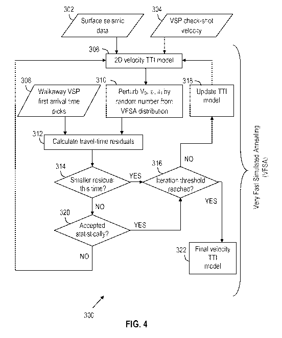
FIG. 4 shows an illustrative TTI model optimization process 300. In process
300, a
2D velocity TTI model 306 receives surface seismic data 302 and VSP check-shot
velocity
304 as inputs. Using the TTI model 306, values for Voi, ci, 6i are perturbed
by random
numbers from a VFSA distribution at block 310. With the resulting values for
Voi, Ei, 6i from
block 310 and with walkaway VSP first arrival time picks 308, travel-time
residuals are
calculated at block 312. If the calculations of block 312 do not result in a
smaller residual
(determination block 314), a determination is made regarding whether the
calculations are
statistically acceptable (determination block 320). If not, the process
returns to block 306. If
the calculations of block 312 are statistically acceptable (determination
block 320) or result in
a smaller residual (determination block 314), a determination is made
regarding whether an
iteration threshold has been reached (determination block 316). If so, the
velocity TTI model
has been finalized (block 322). If the iteration threshold has not been
reached (determination
block 318), the TTI model is updated at block 318 and is used as the TTI model
at block 306
for subsequent operations.
- 12 -
CA 02913242 2015-11-23
WO 2014/204440 PCT/US2013/046269
The operations of process 300 may be based, in part, on a system or vector of
unknowns that the tomographic inversion is optimizing. For some embodiments of
the
disclosed operations, the vector of unknowns is:
X = (VL 'VON'S19L 18N 9 el'L ,eN
)T
(1)
where N is the number of layers to be optimized; Voi is the P-wave velocity
(V0) along the
symmetry axis for layer i; and 6; and Ei are the Thomsen parameters 6 and 6
for layer i.
Further, the operations of process 200 may be based, in part, on an objective
function:
1 R =
E(X)= \I¨E(tiPwk ¨tic.ai) 2 , (2)
R
where R is the total number of arrival time picks; t is the direct arrival
times; subscript i refer
to the ith receiver; and superscripts pick and cal refer to picked and
calculated times. Further,
the operations of process 300 may be based, in part, on a temperature cooling
schedule Tk:
Tk = To exp(¨ck1(2m)) , (3)
where To is the initial temperature, c is a parameter to be used to control
the temperature
schedule and help tune the algorithm for a specific problem, k is the
iteration number in the
optimization, and M is the total number of unknowns. For this application, a
suitable value
for c is approximately 0.05 and for To is 100Ø Further, the operations of
process 300 may be
based, in part, on generation of a random variable u to perturb the X vector.
Considering an
unknown Xik generated at annealing iteration k, xik can be updated to Xik+ 1
as:
min
k+1 = + q(ximax ¨xi ) (4)
where q is a random number and x:n ' and 4¨ are bounds for the unknowns of
layer i,
which is constrained by Xi E [Ximin X7 . The random variable q is generated
from a
- 13 -
CA 02913242 2015-11-23
WO 2014/204440 PCT/US2013/046269
uniformly distributed random number u between zero and one ( u E U[0,1] ) by
the
formula:
q = sgn(u ¨ 0.5)Tk [(1+ y)2U1I _
(5)
Tk
where sgn is the sign function. The random variable lies between -1 and 1 ( q
E [¨ 1, 11 ) and
guarantees the convergence of VFSA.
Further, the operations of process 300 may be based, in part, on iteration
termination
criteria. In at least some embodiments, the termination criteria of the
annealing process are
arbitrary. Reasonable constraints are that the misfit (residuals) remains the
same for a number
of iterations for temperature T close to zero, that the misfit is smaller than
a user-specified
value, and that the total iteration number exceeds the user-specified maximum
iteration. The
process of applying the VFSA technique can thus be halted when any one of
these criteria is
met, yielding the desired anisotropy parameters.
Further, the operations of process 300 may be based, in part, on an accurate
and
efficient TTI ray tracer. In at least some embodiments, the shooting method is
implemented
to provide two-point seismic ray tracing in the TTI media. In the shooting
method, a ray is
shot from a source location with a given shooting direction. Then the shooting
direction is
modified until the ray emerges at the desired receiver location. Once the
raypath is
determined, the seismic travel-times are calculated by integrating the product
of slowness and
raypath segment length along the path using layer group slowness.
A complete raypath is governed by kinematic seismic ray equations with
appropriate
application of Snell's law in the presence of any interface to be traced. In
an anisotropic
medium, the key element is the phase slowness analysis at each layer
interface. FIGS. 5A and
5B show illustrative reflection/transmission angles of slowness vectors in an
anisotropic
medium. In FIGS. 5A and 5B, a ray is incident on the boundary from above, and
phase-
- 14 -
CA 02913242 2015-11-23
WO 2014/204440 PCT/US2013/046269
slowness vectors (for incident, reflected, and transmitted waves) are
coplanar. Denoting the
phase slowness vector as M, the continuity conditions require that
Mi.X=Mr.X=Mt.X, (6)
where X is the unit vector in the x-direction and subscripts i, r, t refer to
incident, reflected,
and transmitted waves, respectively. The group slowness vector W is normal to
the phase
slowness surface. In FIGS. 5A and 5B, the curves represent phase slowness in
the medium of
incidence and transmission, and the Cartesian axes x and z correspond to the
horizontal and
vertical slowness, respectively. In other words, the curves illustrate the
angles for incident,
reflected, and transmitted rays in anisotropic media separated by a
horizontal, planar interface
io using
phase-slowness surface. The M vectors correspond to phase-slowness and W
vectors to
group-slowness; theta (A) and phi (c)) correspond to ray/group angle and phase
angle,
respectively for incident, reflected, and transmitted waves. Note that
ci or
co, for an anisotropic model such as the TTI model described
herein. Once the raypath is determined by the phase slowness analysis, the
seismic
traveltimes are calculated by integrating the product of slowness and raypath
segment length
along the path using layer group slowness.
FIG. 6 shows an illustrative seismic survey recording system having the
receivers 102
coupled to a bus 402 to communicate digital signals to data recording
circuitry 406. Position
information sensors 404 (and optionally sensors for other parameters) are also
coupled to the
data recording circuitry 406 to enable the data recording circuitry to store
additional
information useful for interpreting the recorded data. Illustratively, such
additional
information can include source waveform characteristics, digitization
settings, detected faults
in the system, etc.
Recording circuitry 406 acquires the high speed data stream(s) from receivers
102
onto a nonvolatile storage medium such as a storage array of optical or
magnetic disks. The
- 15 -
CA 02913242 2015-11-23
WO 2014/204440 PCT/US2013/046269
data is stored in the form of (possibly compressed) seismic traces, each trace
being the signal
detected and sampled by a given receiver in response to a given shot. (The
associated shot
and receiver positions are also stored.) Illustrative seismic signals are
shown in FIG. 7. The
signals indicate some measure of seismic wave energy as a function of time
(e.g.,
displacement, velocity, acceleration, pressure), and they are digitized at
high resolution (e.g.,
16 to 32 bits) at a programmable sampling rate (e.g., 400 to 1000 Hz) for a
fixed duration
after each shot (e.g., 30 seconds). Such signals can be grouped in different
ways, and when so
grouped, they are called a "gather". For example, a "common midpoint gather"
is the group
of traces that have a midpoint within a defined region. A "shot gather" is the
group of traces
to recorded for a single firing of the seismic source.
A general purpose data processing system 408 receives the acquired seismic
survey
data from the data recording circuitry 406. In some cases the general purpose
data processing
system 408 is physically coupled to the data recording circuitry and provides
a way to
configure the recording circuitry and perform preliminary processing in the
field. More
typically, however, the general purpose data processing system is located at a
central
computing facility with adequate computing resources for intensive processing.
The survey
data can be transported to the central facility on physical media or
communicated via a
computer network. Processing system 408 includes a user interface having a
graphical
display and a keyboard or other method of accepting user input and/or enabling
users to view
and analyze the subsurface structure images derived from collected seismic
survey data.
The recorded seismic survey data is of little use when maintained in the
format of Fig.
7. Although it is possible to plot the various recorded waveforms side by side
in a plot that
reveals large scale subsurface structures, such structures are distorted and
finer structures
cannot even be seen. Hence the data is processed to create a data volume,
i.e., a three
dimensional array of data values such as that shown in FIG. 8. The data volume
represents
- 16 -
CA 02913242 2015-11-23
WO 2014/204440 PCT/US2013/046269
some seismic attribute throughout the survey region. The three-dimensional
array comprises
uniformly-sized cells, each cell having a data value representing the seismic
attribute for that
cell. Various seismic attributes may be represented, and in some embodiments,
each cell has
multiple data values to represent multiple seismic attributes. Examples of
suitable seismic
attributes include reflectivity, acoustic impedance, acoustic velocity, and
density. The
volumetric data format readily lends itself to computational analysis and
visual rendering,
and for this reason, the data volume may be termed a "three-dimensional image"
of the
survey region.
Fig. 9 shows an illustrative computer system 600 for performing seismic data
o
processing using a TTI model obtained by simultaneous inversion of Vo and the
Thomsen
parameters, E and 8, as described herein. A personal workstation 602 is
coupled via a local
area network (LAN) 604 to one or more multi-processor computers 606, which are
in turn
coupled via the LAN to one or more shared storage units 608. Personal
workstation 602
serves as a user interface to the processing system, enabling a user to load
survey data into
the system, to retrieve and view image data from the system, and to configure
and monitor
the operation of the processing system. Personal workstation 602 may take the
form of a
desktop computer with a graphical display that graphically shows survey data
and images of
the survey region, and with a keyboard that enables the user to move files and
execute
processing software.
LAN 604 provides high-speed communication between multi-processor computers
606 and with personal workstation 602. The LAN 604 may take the form of an
Ethernet
network. Meanwhile, multi-processor computer(s) 606 provide parallel
processing capability
to enable suitably prompt conversion of seismic trace signals into a survey
region image.
Each computer 606 includes multiple processors 612, distributed memory 614, an
internal
bus 616, and a LAN interface 620. Each processor 612 operates on an allocated
portion of the
- 17 -
CA 02913242 2015-11-23
WO 2014/204440 PCT/1JS2013/046269
input data to produce a partial image of the seismic survey region. Associated
with each
processor 612 is a distributed memory module 614 that stores conversion
software and a
working data set for the processor's use. Internal bus 616 provides inter-
processor
communication and communication to the LAN networks via interface 620.
Communication
between processors in different computers 606 can be provided by LAN 604.
Shared storage units 608 may be large, stand-alone information storage units
that
employ magnetic disk media for nonvolatile data storage. To improve data
access speed and
reliability, the shared storage units 608 may be configured as a redundant
disk array. Shared
storage units 608 initially store a velocity data volume and shot gathers from
a seismic
survey. The illumination matrix values and/or reflectivity image volumes can
be stored on
shared storage units 608 for later processing. In response to a request from
the workstation
602, the image volume data can be retrieved by computers 606 and supplied to
workstation
for conversion to a graphical image to be displayed to a user.
FIG. 10 shows an illustrative seismology method 700 that includes collecting
seismic
data (block 702). At block 704, the seismic data is stored. At block 706,
surface seismic data
and VSP check-shot velocity data are input to a TTI model. At block 708, Vo,
c, and 6 are
perturbed by random numbers from a VFSA distribution. At block 710, travel-
time residuals
are determined based on walkaway VSP first arrival time picks and the
perturbed Vo. E, and 6
values. At block 712, TTI model update criteria and termination criteria are
applied.
Examples of TTI model update criteria includes updating the TTI model if the
residuals for
an iteration are smaller than the previous iteration or updating the TTI model
if the residuals
are statistically acceptable. Examples of termination criteria include the
residuals remaining
the same for a number of iterations for temperature T close to zero, the
residuals being
smaller than a threshold value, and/or the total iteration number exceeding a
threshold
number of iterations. The seismology method 700 may be performed by computing
- 18 -
CA 02913242 2015-11-23
WO 2014/204440 PCT/US2013/046269
components of computer system 66, computer system 202, or other computing
components
described herein.
In some embodiments, the method 700 includes additional or alternative steps.
For
example, method 700 may analyze collected seismic data using a TTI model based
on
simultaneous inversion of Vo, e, and 6. The method 700 also may include
related steps such
as determining values for Vo, c, and 6 by minimizing the difference between a
first arrival
pick and a calculated first arrival time. Further, the method 700 may include
receiving VSP
walkaway data and using the VSP walkaway data to minimize the difference
between the first
arrival pick and the calculated first arrival time. Further, the method 700
may include
producing a seismic section from the VSP walkaway data, selecting the first
arrival pick from
the seismic section, and calculating the first arrival time as a travel time
from a seismic
source to a geophone through the TTI model. Further, the method 700 may
include applying
a VFSA process to perform the simultaneous inversion. Further, the method 700
may include
applying, during the VFSA process, an objective function, a temperature
cooling schedule,
and generation of a random variable to perturb values for Vo, 8, and 6.
The tomographic inversion described herein is testable using a synthetic
walkaway
survey. FIG. 11 shows an illustrative synthetic model and seismic survey
geometry composed
of seven layers (Layerl ¨ Layer7). The top layer is ocean water. The
information shown for
each layer includes a layer number, Vo, e, 6, and a tilted angle of the
symmetric axis. These
layer properties may vary for different layers. In the example Layer 1, Vo =
1500m/s, & = 0%,
6 = 0%, and the tilted angle of the symmetric axis = 00. In the example
Layer2, Vo =
2000m/s, c = 0%, 6 = 0%, and the tilted angle of the symmetric axis = 0 . In
the example
Layer3, Vo = 2500m/s, 8 = 5%, 6 = 3%, and the tilted angle of the symmetric
axis = 5 . In the
example Layer4, Vo = 2800m/s, c = 10%, 6 = 5%, and the tilted angle of the
symmetric axis =
80. In the example Layer5, Vo = 3100m/s, E = 15%, 6 =8%, and the tilted angle
of the
- 19 -
CA 02913242 2015-11-23
WO 2014/204440 PCT/1JS2013/046269
symmetric axis = 15 . In the example Layer6, Vo = 3500m/s, 6 = 18%, 8 =10%,
and the tilted
angle of the symmetric axis = 10 . In the example Layer7, Vo = 3800m/s, c =
0%, s3 =0%, and
the tilted angle of the symmetric axis = 0 .
In FIG. 11, the synthetic walkaway survey is composed of 14 shots on the
surface and
300 receivers along the deviated wellbore (not shown in FIG. 11). Further,
shot spacing
increases as a function of distance from the wellhead (i.e., the shot spacing
near the wellhead
is less than the shot spacing far away from the wellhead). The ratio of
maximum shot offset
to maximum receiver depth is limited to around one to avoid header wave and
other
interfering waves.
To obtain check-shot velocity, finite difference forward modeling is conducted
with a
maximum frequency of 75 Hz for the zero offset shot (the nearest one to the
wellhead). FIG.
12 shows an illustrative synthetic waveform of zero offset shot generated by
finite difference
modeling. In FIG. 12, the first arrivals are accurately picked (the top line)
and are used to
generate a check-shot velocity profile which is used as initial velocities for
the tomographic
inversion.
The synthetic waveforms were then loaded into a processing system to generate
a
check-shot velocity profile which shows velocity jumps at depths around 1500
m, 2300 m,
and 3200 m (see FIG. 13). These velocity jumps correspond to the intersection
depths
between the wellbore and layers 3, 4, and 5. Since the check-shot velocity is
accurate for
layers in which receivers are placed, Vo, & and 8 were fixed as their true
values for layers 1, 2,
and 7 during tomographic inversion. In FIG. 13, the left-side graph shows a
traveltime (x-
axis) vesus depth (z-axis) curve 800, and the right-side graph shows three
velocity (x-axis)
vesus depth (z-axis) curves 802, 804, and 806. More specifically, curve 802 is
the average
velocity, curve 804 is the RMS velocity, and curve 806 is the interval
velocity. In some
embodiments, the interval velocity is used as the initial velocity for the TTI
model.
-20-
CA 02913242 2015-11-23
,
WO 2014/204440
PCT/US2013/046269
In the disclosed tomographic inversion, an appropriate value range for Vo, c
and 6 is
set for each layer. The range will be used to constrain the unknowns during
random
perturbation of the ITT model. Values that fall within the range are possible
candidates
during model updates. Table 1 shows a list of initial values for the TTI model
and search
ranges of unknowns. The ranges are defined by table columns of the minimum
values and the
maximum values.
The initial velocity value in Table 1 is the average from the interval
velocity curve
806 of the check-shot velocity profile (FIG. 13). The expected velocity along
the symmetry
axis would not deviate too much from ones along vertical axis. Therefore, the
velocity range
is set as a narrow range (columns 5 and 8 in Table 1). For anisotropic
parameters, the initial
values are set to zero. Based on the regional geology and estimates from
seismic data, the
range for & and 6 (column 6 and 9 for 6, column 7 and 10 for c, Table 1) are
set.
Table 1
:. Initial Values Minimum Values Maximum Values
0
,
ci
,- Vo 6(%) c(%) Vo 6(%) c(%) Vo 6(%) c(%)
3 2600 0 0 2100 0 0 3100 5
10
4 2700 0 0 2200 0 5 3200 10
15
5 3000 0 0 2500 5 10 3500 15
20
6 3500 0 0 3000 5 10 4000 15
20
Table 2
;.., True Inverted
0,
Error Percentage (%)
Values Values
ci
,.-. Vo 6(%) c(%) Vo 6(%) c(%) Vo 6
c
3 2500 3 5 2432 2.81 4.84 -2.7 -6.3
-3.2
4 2800 5 10 2712 5.64 9.23 -3.1 12.8
-7.7
5 3100 8 15 3191 7.13 16.02 2.9 -10.9
6.8
6 3500 10 18 3433 10.67 19.14 -1.9 6.7
6.3
-21-
CA 02913242 2015-11-23
WO 2014/204440 PCT/US2013/046269
Tomographic inversion begins with initial values and ranges listed in Table 1.
After
several trials of VFSA, suitable values can be determined (e.g., c = 0.05, To
= 100.0, and total
iteration = 2000). The final inverted model has a 3.8 ms RMS error as shown in
Table 2
which lists true values, inverted values, and error percentages (the
difference between the true
and the inverted values divided by the true values).
Table 2 entries illustrate that the velocity is well inverted with maximum
error
percentage of 3.1%. The inverted epsilon c is close to the true value with
maximum error
percentage of 7.7%. The inverted delta 6 has larger error percentage (12.8%),
but the absolute
difference is only 0.87%. The absolute difference for the inverted c is small
as well, only
1.14%.
As described herein, TTI tomographic inversion operates to determine the
optimal Vo,
e, and 6 by minimizing the difference between first arrival picks and the
calculated first
arrival times. The VFSA method is used as the parameter estimation engine. As
disclosed
herein, the VFSA method statistically perturbs the model (by adjusting Vo, c,
and 6 of each
layer) and makes statistical decisions on discarding or accepting the
perturbed model.
Compared with many linear or linearized inversions, VFSA has shown a superior
performance and enables global minimum inversion. The final results yielded by
VFSA do
not depend on the initial models used for the inversion. It has been
successfully used in many
geophysical inversion problems. However, there is no mathematic formula to
select suitable
zo parameter values for c, To, and total iteration. These parameters
control the model space
where VFSA searches for the best fits and the model space is problem-
dependent. The rule of
thumb is to do trial runs to find suitable values of these parameters for the
specific problem.
Once determined, these parameters stay fixed. For the disclosed synthetic
examples, c = 0.05,
To = 100.0, and total iteration = 2000 based on several trials.
- 22 -
CA 02913242 2015-11-23
WO 2014/204440 PCT/US2013/046269
The test with noise-free synthetics indicates that both velocity and
anisotropic
parameters are well recovered. It is important to be aware that noise level in
real data may
contaminate the final inverted results. In addition, the uncertainty of first
arrival picks may
increase uncertainty of the final inverted results.
Numerous other modifications, equivalents, and alternatives, will become
apparent to
those skilled in the art once the above disclosure is fully appreciated. For
example, although
at least some software embodiments have been described as including modules
performing
specific functions, other embodiments may include software modules that
combine the
functions of the modules described herein. Also, it is anticipated that as
computer system
performance increases, it may be possible in the future to implement the above-
described
software-based embodiments using much smaller hardware, making it possible to
perform the
described non-physical attribute management operations using on-site systems
(e.g., systems
operated within a well-logging truck located at the reservoir). Additionally,
although at least
some elements of the embodiments of the present disclosure are described
within the context
of monitoring real-time data, systems that use previously recorded data (e.g.,
"data playback"
systems) and/or simulated data (e.g., training simulators) are also within the
scope of the
disclosure. It is intended that the following claims be interpreted to embrace
all such
modifications, equivalents, and alternatives where applicable.
-23 -