Note : Les descriptions sont présentées dans la langue officielle dans laquelle elles ont été soumises.
CA 02920169 2016-02-01
WO 2015/038102 PCT/US2013/059066
SURFACE CALIBRATION OF A WELLBORE RESISTIVITY LOGGING TOOL
HELD OF THE DISCLOSURE
The present disclosure relates generally to calibration techniques for
wellbore
logging tools and, more specifically, to a surface calibration method for a
resistivity
logging tool.
BACKGROUND
Among all logging tools deployed in the wellbore, resistivity tools provide
the
largest depth of detection. As a result, they have been extensively used for
detecting
formation layer boundaries in applications such as landing or well placement.
Moreover,
io such logging tools are utilized to acquire various other characteristics
of earth formations
traversed by the wellbore and data relating to the size and configuration of
the wellbore
itself. The collection of information relating to downhole conditions,
commonly referred to
as "logging," can be performed by several methods including wireline logging
and "logging
while drilling" ("LWD").
The depth of detection provided by the logging tool is directly proportional
to the
distance between the transmitter and the receiver. As a result, most of the
deep reading
tools have very large distance between them. For example, some deep
resistivity reading
tools can be as long as 50-100 feet, and they operate at frequencies lower
than 8 KHz to
compensate for the geometrically increasing attenuation at larger transmitter
receiver
zo separations. In contrast, the standard, shallower, tools have a range of
about 20 feet and
they are optimized for placement of wells in reservoirs within about 10 feet
from the top or
bottom boundary of the reservoir rock.
The required distances between the transmitters and receivers along deep
reading
tools create problems in calibration since most of the conventional
calibration methods (air
hang, test tank, or oven, for example) require a certain stand-off from any
nearby objects
that might interfere with the calibration measurement signals. As a result, it
is impractical
to apply these conventional calibration techniques to a deep reading
resistivity tool since
the tool's sensitive volume is too large and, thus, it is not feasible to have
facilities big
enough to fully contain the tools.
Accordingly, there is a need in the art for a practical technique in which to
calibrate
a deep reading resistivity logging tool.
1
CA 02920169 2016-02-01
WO 2015/038102 PCT/1JS2013/059066
BRIEF DESCRIPTION OF THE DRAWINGS
FIG. 1 illustrates a logging tool situated on a stand which is calibrated
according to
certain illustrative methodologies of the present disclosure;
FIGS. 2A and 2B illustrate a resistivity logging tool, utilized in an LWD and
wireline application, respectively, according certain illustrative embodiments
of the present
disclosure;
FIG. 2C shows a block diagram of circuitry embodied within a logging tool
necessary to acquire the formation measurement signals, according to certain
illustrative
io embodiments of the present disclosure;
FIG. 3A is a flow chart detailing a surface calibration method according to
certain
illustrative methodologies of the present disclosure;
FIG. 38 is a flow chart detailing a surface calibration methodology utilized
at block
312 of method 300 to calculate receiver coefficients, according to one or more
alternative
illustrative methodologies of the present disclosure;
FIG. 3C is a flow chart detailing a surface calibration methodology utilized
at block
312 of method 300 to calculate transmitter coefficients, according to one or
more
alternative illustrative methodologies of the present disclosure;
FIG. 4 is a flow chart of a method detailing application of the calibration
coefficients to modeling, according to one or more illustrative methodologies
of the present
disclosure;
FIG. 5 is a flow chart of a method detailing application of the calibration
coefficients to real measurements, according to one or more alternative
illustrative
methodologies of the present disclosure;
FIGS. 6A-D illustrates graphs A-D which show modeling results for the
calibration
methods described herein;
FIGS 7A-D are graphs showing the logging tool receiver and transmitter
calibration
sensitivity to eccentricity effects as a function of loop position, according
to certain
illustrative embodiments of the present disclosure; and
FIGS. 8A-D are graphs showing the logging tool receiver and transmitter
calibration sensitivity to loop tilt angle deviation as a function of loop
position, according
to certain illustrative embodiments of the present disclosure.
2
CA 02920169 2016-02-01
WO 2015/038102 PCT/US2013/059066
DESCRIPTION OF ILLUSTRATIVE EMBODIMENTS
Illustrative embodiments and related methodologies of the present disclosure
are
described below as they might be employed in a surface calibration methodology
for use
with wellbore resistivity logging tools. In the interest of clarity, not all
features of an actual
implementation or methodology are described in this specification. It will of
course be
appreciated that in the development of any such actual embodiment, numerous
implementation-specific decisions must be made to achieve the developers'
specific goals,
such as compliance with system-related and business-related constraints, which
will vary
io from one implementation to another. Moreover, it will be appreciated
that such a
development effort might be complex and time-consuming, but would nevertheless
be a
routine undertaking for those of ordinary skill in the art having the benefit
of this
disclosure. Further aspects and advantages of the various embodiments and
related
methodologies of the disclosure will become apparent from consideration of the
following
description and drawings.
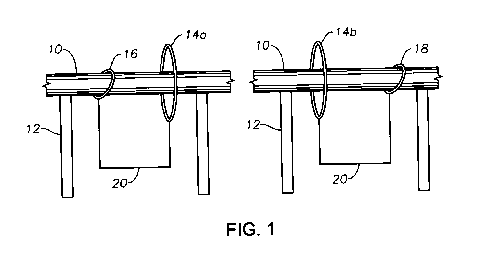
FIG. 1 illustrates a logging tool situated on a stand which is calibrated
according to
an exemplary methodology of the present disclosure. As described herein,
illustrative
embodiments of the present disclosure describe various methodologies for
surface
calibration of resistivity logging tools. A logging tool 10 is first
positioned on a stand 12.
Alternatively, logging tool 10 may be suspended or otherwise secured at a
surface location.
Loops 14 (i.e., transmitter loop 14a or receiver loop 14b) are positioned
adjacent to the tool
receiver 16 and transmitter 18, respectively. For example, loops 14 may be a
distance of 10
to 20 feet in some embodiments. In certain embodiments, separate external
transmitter and
receiver loops are used for calibration. Such an embodiment will be especially
useful for a
modular tool, as shown in FIG. 1, where the transmitter and receiver of a deep
reading tool
are on physically separate pieces of a collar. However, the present disclosure
is also
applicable to unified logging tools. Nevertheless, surface calibration of the
transmitter and
receiver can be conducted separately, which requires less physical space and
clearance for
the measurements.
As further shown in FIG. 1, in order to calibrate transmitter 18, external
calibrated
receiver loop 14b is placed in the vicinity of transmitter 18 to thereby
record signals
emanating from transmitter 18. The measured signals are then compared to
simulated
3
CA 02920169 2016-02-01
WO 2015/038102 PCT/US2013/059066
signals and, as a result of the comparison, calibration coefficients for
transmitter 18 are
determined. Calibration of tool receiver 16 is accomplished in like manner
through use of
loop transmitter 14a. In certain embodiments, synchronization (to calibrate
phase) between
tool transmitter 18/receiver 16 and their respective loop receiver
14b/transmitter 14a may
be accomplished by placing a synchronization line 20 between them. Line 20 may
be
wired or wireless.
Thereafter, the tool is deployed downhole and formation measurements are taken
as
shown in FIGS. 2A and 2B. FIGS. 2A and 2B illustrate a resistivity logging
tool, utilized
in an LWD and wireline application, respectively, according certain
illustrative
io embodiments of the present disclosure. Once deployed, the calibration
coefficients for tool
transmitter 18 and receiver 16 calculated at the surface are applied to real
signals obtained
downhole to thereby calibrate the measurements. Thereafter, the calibrated
measurement
signal is inverted to generate desired petrophysical characteristics of the
borehole and
surrounding geological formation (i.e., formation parameters) related to
electrical or
geological properties of the formation such as, for example, layer
resistivities, distances or
direction to layer boundaries, 2D shape of arbitrary layer boundaries, or 3D
distribution of
formation resistivities. In an alternative mode of application of calibration,
the calibration
may be applied to the model data in inversion instead. Accordingly, wellbore
operations
may be conducted based upon the formation parameters such as, for example,
drilling, well
placement, landing or geosteering operations.
FIG. 2A illustrates a drilling platform 2 equipped with a derrick 4 that
supports a
hoist 6 for raising and lowering a drill string 8. Hoist 6 suspends a top
drive 11 suitable for
rotating drill string 8 and lowering it through well head 13. Connected to the
lower end of
drill string 8 is a drill bit 15. As drill bit 15 rotates, it creates a
wellbore 17 that passes
through various formations 19. A pump 21 circulates drilling fluid through a
supply pipe
22 to top drive 11, down through the interior of drill string 8, through
orifices in drill bit
15, back to the surface via the annulus around drill string 8, and into a
retention pit 24. The
drilling fluid transports cuttings from the borehole into pit 24 and aids in
maintaining the
integrity of wellbore 16. Various materials can be used for drilling fluid,
including, but not
limited to, a salt-water based conductive mud.
The logging tool 10 is integrated into the bottom-hole assembly near the bit
15. In
this illustrative embodiment, logging tool 10 is an LWD tool; however, in
other illustrative
4
CA 02920169 2016-02-01
WO 2015/038102 PCT/1JS2013/059066
embodiments, logging tool 10 may be utilized in a wireline or tubing-convey
logging
application. Logging tool 10 may be, for example, an ultra-deep reading
resistivity tool.
Alternatively, non-ultra-deep resistivity logging tools may also be utilized
in the same drill
string along with the deep reading logging tool. Illustrative logging tools
include, for
example, Halliburton Energy Services, Co.'s INSITE ADRTM resistivity tool or
the LOGIQ
ACRtTM System. Persons ordinarily skilled in the art having the benefit of
this disclosure
will realize there are a variety of resistivity logging tools which may be
utilized within the
present disclosure. Moreover, in certain illustrative embodiments, logging
tool 10 may be
adapted to perform logging operations in both open and cased hole
environments.
Furthermore, in certain embodiments, the measurement signals utilized in the
calibration
process may have originated from different boreholes, preferably in the same
region of
earth where a strong relationship exists between the boreholes.
Still referring to FIG. 2A, as drill bit 15 extends wellbore 17 through
formations 19,
logging tool 10 collects measurement signals relating to various formation
properties, as
well as the tool orientation and various other drilling conditions. In certain
embodiments,
logging tool 10 may take the form of a drill collar, i.e., a thick-walled
tubular that provides
weight and rigidity to aid the drilling process. However, as described herein,
logging tool
10 includes an induction or propagation resistivity tool to sense geology and
resistivity of
formations. A telemetry sub 28 may be included to transfer images and
measurement
data/signals to a surface receiver 30 and to receive commands from the
surface. In some
embodiments, telemetry sub 28 does not communicate with the surface, but
rather stores
logging data for later retrieval at the surface when the logging assembly is
recovered.
Still referring to FIG. 2A, logging tool 10 includes a system control center
("SCC"),
along with necessary processing/storage/communication circuitry, that is
communicably
coupled to one or more sensors (not shown) utilized to acquire formation
measurement
signals reflecting formation parameters. In certain embodiments, once the
measurement
signals are acquired, the SCC calibrates the measurement signals and
communicates the
data back uphole and/or to other assembly components via telemetry sub 28. In
an
alternate embodiment, the system control center may be located at a remote
location away
from logging tool 10, such as the surface or in a different borehole, and
performs the
processing accordingly. These and other variations within the present
disclosure will be
readily apparent to those ordinarily skilled in the art having the benefit of
this disclosure.
5
CA 02920169 2016-02-01
WO 2015/038102 PCT/1JS2013/059066
The logging sensors utilized along logging tool 10 are resistivity sensors,
such as,
for example, magnetic or electric sensors, and may communicate in real-time.
Illustrative
magnetic sensors may include coil windings and solenoid windings that utilize
induction
phenomenon to sense conductivity of the earth formations. Illustrative
electric sensors may
s include electrodes, linear wire antennas or toroidal antennas that
utilize Ohm's law to
perform the measurement. In addition, the sensors may be realizations of
dipoles with a
azimuthal moment direction and directionality, such as tilted coil antennas.
In addition, the
logging sensors may be adapted to perform logging operations in the up-hole or
downhole
directions. Telemetry sub 28 communicates with a remote location (surface, for
example)
io using, for example, acoustic, pressure pulse, or electromagnetic
methodologies, as will be
understood by those ordinarily skilled in the art having the benefit of this
disclosure.
As described above, logging tool 10 is, in this example, a deep sensing
induction or
propagation resistivity tool. As will be understood by those ordinarily
skilled in the art
having the benefit of this disclosure, such tools typically include
transmitter and receiver
is coils that are axially separated along the wellbore. The transmitter
coils generate
alternating displacement currents in the formation that are a function of
conductivity. The
alternating currents generate voltage at the receiver coil. In addition to the
path through the
formation, a direct path from the transmitter to receiver also exists. In
induction tools,
signal from such path can be eliminated by the use of an oppositely wound and
axially
20 offset "bucking" coil. In propagation tools, phase and amplitude of the
complex-valued
voltage can be measured at certain operating frequencies. In such tools, it is
also possible
to measure phase difference and amplitude ratio between two axially spaced
receivers. The
phases, phase differences, amplitudes or amplitude ratios can all be
calculated from
complex-valued voltage measurements at the receivers. Furthermore, pulse-
excitation and
25 time-domain measurement signals can be used in the place of frequency
domain
measurement signals. Such measurement signals can be transformed into
frequency
measurements by utilizing a Fourier transform. The calibration methods
described below
are applicable to all of these signals and no limitation is intended with the
presented
examples. Generally speaking, a greater depth of investigation can be achieved
using a
30 larger transmitter-receiver pair spacing, but the vertical resolution of
the measurement
signals may suffer. Accordingly, logging tool 10 may employ multiple sets of
transmitters
6
CA 02920169 2016-02-01
WO 2015/038102 PCT/US2013/059066
or receivers at different positions along the wellbore to enable multiple
depths of
investigation without unduly sacrificing vertical resolution.
FIG. 2B illustrates an alternative embodiment of the present invention whereby
a
surface calibrated wireline logging obtains and calibrates measurement
signals. At various
times during the drilling process, drill string 8 may be removed from the
borehole as shown
in FIG. 2B. Once drill string 8 has been removed, logging operations can be
conducted
using a wireline logging sonde 34, i.e., a probe suspended by a cable 41
having conductors
for transporting power to the sonde 34 and telemetry from sonde 34 to the
surface. The
wireline logging sonde 34 includes the logging tool 10 and may have pads
and/or
io centralizing springs to maintain the tool near the axis of wellbore 17
as the tool 10 is pulled
uphole. Logging sonde 34 can include a variety of sensors including a multi-
array laterolog
tool for measuring formation resistivity. A logging facility 43 collects
measurements from
the logging sonde 34, and includes a computer system 45 for processing and
storing the
measurements gathered by the sensors.
Is FIG. 2C shows a block diagram of circuitry 200 embodied within logging
tool 10
(or other logging tools described herein such as, for example, sonde 34)
necessary to
acquire the formation measurement signals, according to certain illustrative
embodiments
of the present disclosure. Logging tool 10 is comprised of one or more
transmitters
T I ...TN and receivers R1...RN, and associated antennas, placed within
grooves along
20 logging tool 10, which may comprise, for example, magnetic dipole
realizations such as
coiled, tilted coil, solenoid, etc. During logging operations, pulsed or
steady-state signals
are generated at the transmitting antennas which interact with the formation
and layer
boundaries in the vicinity of logging tool 10 to produce electrical signals
(i.e., measurement
signals) that are picked up by the receivers. Utilizing data acquisition unit
27, system
25 control center 25 then collects and calibrates the formation measurement
signal using the
methodologies described herein. Thereafter, system control center 25 records
the
measurement signal data to buffer 29, applies data pre-processing (using data
processing
unit 30) for reducing the bandwidth requirement, and then communicates the
data to a
remote location (surface, for example) using communication units 32 (telemetry
sub 28, for
30 example). As previously described, however, the uncalibrated formation
measurement
signals may be transmitted to a remote location where the calibration is then
conducted.
Calibration of the formation measurement signals may be conducted remotely.
However,
7
CA 02920169 2016-02-01
WO 2015/038102 PCT/US2013/059066
in those embodiments in which the calibration is conducted by logging tool 10,
tool
response times may be improved and telemetry bandwidth to other tools in the
bottom hole
assembly may be increased.
Although not shown in FIG. 2C, circuitry 200 includes at least one processor
embodied within system control center 25 and a non-transitory and computer-
readable
storage, all interconnected via a system bus. Software instructions executable
by the
processor for implementing the illustrative calibration methodologies
described herein in
may be stored in local storage or some other computer-readable medium. It will
also be
recognized that the calibration software instructions may also be loaded into
the storage
io from a CD-ROM or other appropriate storage media via wired or wireless
methods.
Moreover, those ordinarily skilled in the art will appreciate that various
aspects of
the disclosure may be practiced with a variety of computer-system
configurations,
including hand-held devices, multiprocessor systems, microprocessor-based or
programmable-consumer electronics, minicomputers, mainframe computers, and the
like.
Any number of computer-systems and computer networks are acceptable for use
with the
present disclosure. The disclosure may be practiced in distributed-computing
environments
where tasks are performed by remote-processing devices that are linked through
a
communications network. In a distributed-computing environment, program
modules may
be located in both local and remote computer-storage media including memory
storage
devices. The present disclosure may therefore, be implemented in connection
with various
hardware, software or a combination thereof in a computer system or other
processing
system.
System control center 25 may further be equipped with earth modeling
capability in
order to provide and/or transmit subsurface stratigraphic visualizations
including, for
example, geo science interpretation, petroleum system modeling, geochemical
analysis,
stratigraphic gridding, facies, net cell volume, and petrophysical property
modeling. In
addition, such earth modeling capability may model well traces, perforation
intervals, as
well as cross-sectional through the facies and porosity data. Illustrative
earth modeling
platforms include, for example, DecisionSpace , as well as its PerfWizarde
functionality,
which is commercially available through Landmark Graphics Corporation of
Houston,
Texas. However, those ordinarily skilled in the art having the benefit of this
disclosure
8
CA 02920169 2016-02-01
WO 2015/038102 PCT/US2013/059066
realize a variety of other earth modeling platforms may also be utilized with
the present
disclosure.
FIG. 3A is a flow chart detailing a surface calibration method 300 according
to
certain illustrative methodologies of the present disclosure. Method 300 is a
generalized
methodology of the more detailed methodologies described later. At block
302(i), a loop
transmitter is positioned adjacent to the receiver logging tool such as, for
example, as
shown in FIG. 1. At block 302(ii), a loop receiver is positioned adjacent to
the logging tool
transmitter. In certain illustrative embodiments, the loop transmitter is
separate from the
loop receiver. As will be understood by those ordinarily skilled in the art
having the
benefit of this disclosure, the loop transmitter/receivers and tool
transmitters/receivers
described herein are coupled to circuitry that provides excitation signals
and/or data
acquisition ability necessary to conduct the calibration techniques. For
purposes of the
following description, such circuitry will be referred to as the system
control center
("SCC") 25.
At block 304(i), SCC 25 excites the transmitter loop to transmit a first
signal. At
block 304(ii), SCC 25 excites the logging tool transmitter to transmit a
second signal. At
block 306(i), the first signal is measured by the logging tool receiver. At
block 306(ii), the
second signal is measured by the loop receiver. The loop transmitter is
calibrated by
utilizing a stable and known receiver, and loop receiver is calibrated by
utilizing a stable
and known source. The loop transmitter and loop receiver circuitry may be
designed to be
very stable references since they are at the surface and they don't have to
operate at harsh
environments, and they can preserve their stability for an extended period of
time. At
block 308(i), SCC 25 simulates (or models) a third signal, while at block
308(ii), SCC 25
simulates a fourth signal. The simulations are conducted using parameters of
the
environment in which the calibration setup is deployed, which is usually a
workshop at the
surface. Since the distance between the transmitters and receivers are small,
sensitivity
range of the measurements are small, which means details of the environment
such as walls
of the workshop, nearby benches, do not need to be included in the model.
At block 310(i), SCC 25 compares the measured first signal with the simulated
third signal. At block 310(ii), SCC 25 compares the measured second signal
with the
simulated fourth signal. At block 312, SCC 25 then calculates the calibration
coefficients
for the logging tool based upon the comparisons of blocks 310(i) and 310(ii).
To achieve
9
CA 02920169 2016-02-01
WO 2015/038102 PCT/US2013/059066
this, SCC 25 utilizes one of the illustrative calibration techniques described
below to
calculate the calibration coefficients. Thereafter, at block 314, SCC 25
utilizes the
calibration coefficients to calibrate the logging tool and/or obtained
measurements.
In certain illustrative methodologies, at block 312, SCC 25 calculates the
calibration coefficients for the logging tool receiver and the logging tool
transmitter
separately. Here, SCC 25 calculates the calibration coefficients for the
logging tool
receiver based upon the comparison of the measured first signal and the
simulated third
signal. In addition at block 312, SCC calculates the calibration coefficients
for the logging
tool transmitter based upon the comparison of the measured second signal and
the
simulated fourth signal.
Referring back to block 314, in certain illustrative embodiments, calibrating
the
logging tool further includes deploying the logging tool downhole and
obtaining a fifth
signal (or measurement) representative of a real formation characteristic
using the logging
tool receiver. Thereafter, the fifth signal is calibrated using the
calibration coefficients
calculated in block 312. Here, in one example, the calibration coefficients of
the logging
tool transmitter and receiver are combined in order to calibrate the fifth
signal.
The calibrated fifth signal is then then inverted to produce desired formation
parameters which are mainly related to electrical or geological properties of
the formation,
such as layer resistivities, distances, direction to layers. Illustrative
inversion techniques
employed may include, for example, pattern matching or iterative methods
utilizing look-
up tables or numerical optimization based on forward modeling, as will be
understood by
those ordinarily skilled in the art having the benefit of this disclosure.
Illustrative
formation parameters may include, for example, layer resistivities, layer
positions, layer
boundary shapes, 3D resistivity distribution, dip angle, strike angle,
borehole radius,
borehole resistivity, eccentricity or eccentricity azimuth. Moreover, in
certain illustrative
embodiments, SCC 25 may also output the calibrated fifth signal(s) in a
variety of forms
such as, for example, simply transmitting the data to a remote location
(surface, for
example) or outputting the data in a report or geological model.
Thereafter, a variety of wellbore operations may be performed based upon the
formation data. For example, drilling decisions such as landing, geosteering,
well
placement or geostopping decisions may be performed. In the case of landing,
as the
bottom hole assembly drilling the well approaches the reservoir from above,
the reservoir
CA 02920169 2016-02-01
WO 2015/038102 PCUUS2013/059066
boundaries are detected ahead of time, thus providing the ability to steer the
wellbore into
the reservoir without overshoot. In the case of well placement, the wellbore
may be kept
inside the reservoir at the optimum position, preferably closer to the top of
the reservoir to
maximize production. In the case of geostopping, drilling may be stopped
before
penetrating a possibly dangerous zone.
The foregoing method 300 embodies a general overview of the illustrative
methodologies of the present disclosure. Below, more detailed alternative
methodologies
of the present disclosure will be described.
FIG. 3B is a flow chart detailing a surface calibration methodology utilized
at block
io 312 of method 300 to calculate receiver coefficients, according to one
or more alternative
illustrative methodologies of the present disclosure. As described above,
calibration
coefficients may be separately calculated for the logging tool receiver and
transmitter. In
one such methodology, calculating the calibration coefficients for the logging
tool receiver
are detailed beginning at block Ra(i), wherein, via a user interface, SCC 25
is instructed to
select one or more transmitter loop configuration(s) represented by:
Lj = LT, LA] Eq.(1),
where LP i are the transmitter loop positions along the logging tool, LT i are
the transmitter
loop tilt angles, and LA i are the transmitter loop azimuth angles. Here,
there are at least
two reasons why multiple transmitter loop configurations may be utilized: (i)
to allow for
enough number of measurements to solve for all unknown receiver configuration
parameters; and (ii) to optimize sensitivity to receiver configuration
parameters (one
particular measurement may have sensitivity to one parameter, but not
necessarily others).
Note, as described above in method 300, the measured first signal is obtained
using the
selected transmitter loop configuration(s). It is noted here that some
additional loop
configuration parameters may also be included, such as, for example, loop
eccentricity
distance and loop eccentricity direction, which describe how the loop is
eccentered with
respect to the tool. In addition, more parameters may be required for a non-
circular or
elliptical loop. For simplicity, the discussion below will be made based on
the three
selected parameters. However, the discussion below is also applicable to any
set of loop
parameters that may be utilized.
At block Rb(i), through activation of the selected logging tool receiver, SCC
25
acquires a real calibration response using the selected transmitter loop
configuration(s).
11
CA 02920169 2016-02-01
WO 2015/038102 PCT/US2013/059066
The resulting real calibration response of the loop transmitter to receiver
may be
represented by:
Xi = REAL_LR(Li,RJ) Eq.(2).
At block Ra(ii), SCC 25 is again instructed, via a user interface, to select
one or
more logging tool receiver configuration(s) R = [RC, RP, RTJ, RAJ], where RC
is the
receiver complex gain, RP J are the receiver positions along the logging tool,
RTJ are the
receiver tilt angles, and RAJ are the receiver azimuth angles. Here, an
initial guess on
receiver configurations may be made. Since receivers are built based on an
ideal intended
design, a good initial guess is typically available. Note also, as described
above in method
io 300, the third signal is simulated using the selected receiver
configuration(s).
At block Rb(ii), SCC 25 simulates the selected transmitter loop
configuration(s) of
block Ra(i) with the selected logging tool receiver configurations of block
Ra(ii), SCC
acquires a simulated response represented by:
Mi = MODEL_LR(Li,RJ) Eq.(3),
which is the analytical ideal response model of the receiver to the
transmitter loop.
Thereafter, at block Rc, SCC 25 determines the logging tool receiver
configuration that
minimizes the mismatch between the real (i.e., measured first signal) and
simulated (i.e.,
simulated third signal) responses. The mismatch may be defined as the summed
squared
difference of the signals, or as the summed absolute value of the difference
in the signals,
as would be understood by those ordinarily skilled in the art having the
benefit of this
disclosure. Therefore, the receiver configuration that minimizes the mismatch
may be
represented by:
= argmin(sumlXi - Mil) Eq.(4).
SCC 25 then utilizes the determined logging tool receiver configuration(s) as
the receiver
calibration coefficients. Here, more specifically, based on a comparison
between real
measurements acquired using the selected transmitter loop configurations and
the logging
tool receiver and the resulting simulation, logging tool receiver
configuration parameters
are inverted and obtained through an inversion process. There are a variety of
inversion
techniques which may be utilized, as will be understood by those ordinarily
skilled in the
art having the benefit of this disclosure. As an example variation, different
weights may be
used in the sum in Eq 4 for different terms.
12
CA 02920169 2016-02-01
WO 2015/038102 PCT/US2013/059066
FIG. 3C is a flow chart detailing a surface calibration methodology utilized
at block
312 of method 300 to calculate transmitter coefficients, according to one or
more
alternative illustrative methodologies of the present disclosure. As detailed
below, the
transmitter calibration method is analogous to the receiver calibration method
of FIG. 3B.
At block Ta(i), wherein, via a user interface, SCC 25 is instructed to select
one or more
receiver loop configuration(s) represented by:
= [LPi, LT, LA] Eq.(5),
where LP i are the receiver loop positions along the logging tool, LT i are
the receiver loop
tilt angles, and LA i are the receiver loop azimuth angles. Thus, as described
above in
io method 300, the measured second signal is obtained using the selected
receiver loop
configuration(s). It is noted here that some additional loop configuration
parameters may
also be included, such as, for example, loop eccentricity distance and loop
eccentricity
direction, which describe how the loop is eccentered with respect to the tool.
In addition,
more parameters may be required for a non-circular or elliptical loop. For
simplicity, the
discussion below will be made based on the three selected parameters. However,
the
discussion below is also applicable to any set of loop parameters that may be
utilized.
At block Tb(i), through activation of the selected receiver loop
configuration(s),
SCC 25 acquires a real calibration response using the logging tool
transmitter. The
resulting real calibration response Xi of the transmitter to receiver loop may
be represented
by:
Xi = REAL_TL(Li,Ti) Eq.(6).
At block Ta(ii), SCC 25 is again instructed, via a user interface, to select
one or
more logging tool transmitter configuration(s) Tj = [TCj, TPj, TT, TA], where
Tci is the
transmitter complex gain, TPi are the transmitter positions along the logging
tool, TTi are
the transmitter tilt angles, and TAi are the transmitter azimuth angles. Here,
an initial guess
on transmitter configurations may be made. Since transmitters are built based
on an ideal
intended design, a good initial guess is typically available. Note also, as
described above in
method 300, the fourth signal is simulated using the selected receiver
configuration(s).
At block Tb(ii), SCC 25 simulates the selected receiver loop configuration(s)
of
block Ta(i) with the selected logging tool transmitter configurations of block
Ta(ii), SCC
acquires a simulated response Mi represented by:
= MODEL_TL(Li,T) Eq.(7),
13
CA 02920169 2016-02-01
WO 2015/038102 PCT/US2013/059066
which is the analytical ideal response model of the transmitter to the
receiver loop.
Thereafter, at block Tc, SCC 25 determines the logging tool transmitter
configuration that
minimizes the mismatch between the real Xi (i.e., measured second signal) and
simulated
Mi (i.e., simulated fourth signal) responses as represented by:
Tisin = argmin(sumlXi - Fx1.(8).
SCC 25 then utilizes the determined logging tool transmitter configuration(s)
as the
transmitter calibration coefficients. Here, based on a comparison between
real
measurements acquired using the selected receiver loop configurations and the
logging tool
transmitter and the resulting simulation, logging tool transmitter
configuration parameters
to are inverted and obtained through an inversion process.
In certain illustrative embodiments, after the calibration coefficients for
both the
logging tool transmitter and receiver are obtained by SCC 25, they can be
stored within the
logging tool circuitry itself or at a remote location such as the surface.
Thereafter, the
calibration coefficients are applied as described below.
FIG. 4 is a flow chart of a method 400 detailing application of the
calibration
coefficients to modeling, according to one or more illustrative methodologies
of the present
disclosure. After the logging tool has been calibrated (i.e., the calibration
coefficients
obtained), the logging tool is deployed downhole along a formation at block
402. At block
404(i), SCC 25 then activates the tool and obtains a fifth signal representing
one or more
real formation characteristics F of the surrounding formation. At block
404(ii), SCC 25
simulates the logging tool using simulated formation characteristics P and the
transmitter
and receiver configurations determined at block 312 (Tc,Rc) above to thereby
obtain a
simulated sixth signal. Here, the simulated sixth signal may be represented
as:
S = MODEL DOWNHOLE (P, Tjsin, RA) Eq.(9).
At block 406, SCC 25 then iteratively determines the simulated formation
parameters P that minimize the mismatch between the real F (i.e., fifth
signal) and
simulated S (i.e., simulated sixth signal), as represented by:
Poi = argmin(sumlF - SI) Eq.(10).
Finally, SCC 25 obtains the simulated parameters as a result of inversion.
Thus, method
400 describes application of the calibration coefficients to modeling, as
opposed to
application of the calibration coefficients to actual measurements (as will be
described in
FIG. 5). Method 400 is simple and efficient in application to allow for
correction of the
14
CA 02920169 2016-02-01
WO 2015/038102 PCT/US2013/059066
inversion outputs. As described below, the methodology of FIG. 5 allows for
correction of
the real measurements.
FIG. 5 is a flow chart of a method 500 detailing application of the
calibration
coefficients to real measurements, according to one or more alternative
illustrative
methodologies of the present disclosure. After the logging tool receiver and
transmitter
calibration coefficients of block 312 have been obtained, SCC 25 determines
(e.g., uploads)
the intended logging tool transmitter and receiver configurations at blocks
502(i) and
502(ii), respectively. The intended configurations are the known ideal
configurations that
were targeting during fabrication. Here, the intended transmitter
configurations are
lo represented by:
IT = [ITC, ITPi, ITT], ITAJ, Eq.(11),
where IT is the transmitter gain, ITPJ are the transmitter positions along the
tool, ITTi are
the transmitter tilt angles, and ITAi are the transmitter azimuth angles. The
intended
receiver configurations are represented by:
1R = [IRCi, IRPj, IRTi, IRA] Eq.(12),
where IRCi is the receiver gain, IRPj are the receiver positions, IRTi are the
receiver tilt
angles, and IRAj are the receiver azimuth angles. As mentioned for the loop
configuration
parameters above, the number of parameters that are used for the logging tool
transmitter
and receiver parameters can also be varied. The discussion below is made for
the above set
zo of parameters, however it could be extended to any other set of
parameters. As an
example, the number of parameters can be reduced by removing those parameters
that are
believed to not vary as much as others based on the particular mechanical
design of the
tool.
At block 504, SCC 25 maps the intended transmitter and receiver configurations
to
the transmitter and receiver configurations (Tc,Rc) determined at block 312.
The MAP
may be represented as:
MAP(MODEL_DOWNHOLE(P, Tjsiõ, R)) = MODEL_DOWNHOLE(P,ITJ,IRi)
Eq.(13).
Here, a SCC 25 computes a correction mapping MAP that takes the real
measurements and
maps them to the intended measurements. Ultimately, this map is used to
correct the real
formation measurements before they are used in the inversion. Thereafter, at
block 506,
the logging tool is deployed downhole. At block 508(i), SCC 25 obtains a fifth
signal
CA 02920169 2016-02-01
WO 2015/038102 PCT/US2013/059066
representing real formation characteristics F using the logging tool. At block
508(ii), SCC
25 simulates the logging tool using simulated formation characteristics P and
the
determined transmitter and receiver configurations Tc,Rc to thereby obtain a
simulated
sixth signal, as represented by:
S = MODEL DOWNHOLE (P, IT, IRJ) Eq.(14).
Finally, at block 510, SCC 25 determines the simulated formation
characteristics P that
minimize the mismatch between the real F (i.e., fifth signal) and simulated S
(i.e.,
simulated sixth signal) signals as represented by:
Psin = argmin(sumIMAP(F) - Eq.(15).
to Accordingly, SCC 25 corrects the real formation measurements before they
are utilized in
the inversion.
FIG. 6A-D illustrate graphs that show modeling results for the calibration
methods
described above. FIG. 6A shows the received signal at the loop receiver due to
the tool
transmitter, while FIG. 6B shows the received signal at the tool receiver due
to loop
transmitter. As expected, signal levels are very high and they decrease as
measurements are
taken from farther away. In these examples, signals are observed to be
detectable at all
distances considered. FIGS. 6C and 6D show the percentage change in the signal
to loop
position per an inch of displacement. In these examples, it can be seen that
any position
that is as least 10 feet away can be used to accurately calculate the
calibration coefficients.
At this range, less than 2% error per 1 inch of positioning error is
generated. Also, as
shown, the sweet spot for the measurement is about 50 feet away from the
sensor provided
that physical space is available. Here, to obtain the calibration
coefficients, one or more
points along the graphs may be compared; however, ideally, the max points at
50 feet
would be utilized.
FIGS. 7A-D are graphs showing the logging tool receiver and transmitter
calibration sensitivity to eccentricity (i.e., off-ccntering of loop) effects
as a function of
loop position, according to certain illustrative embodiments of the present
disclosure. FIG.
7A shows the tool receiver signal induced by the transmitter loop as a
function of
transmitter loop position in feet, and FIG. 7C shows the respective percentage
error. FIG.
7B shows the receiver loop signal induced by the tool transmitter as a
function of receiver
loop position in feet, and FIG. 7D shows the respective percentage error. lt
can be seen
from FIGS. 7A-D that, even when near the transmitter or receiver positions (at
z=50 and
16
CA 02920169 2016-02-01
WO 2015/038102 PCT/US2013/059066
z=0 feet, respectively), deviations in loop eccentricity produces less than
0.6% change in
the received signal for 2 inch off-centering. It can be concluded from these
results that
eccentricity does not need to be controlled precisely and included as a
parameter to
modeling as long as the error can be kept within 2 inch of eccentricity.
FIGS. 8A-D illustrate graphs showing the logging tool receiver and transmitter
calibration sensitivity to loop tilt angle deviation as a function of loop
position, according
to certain illustrative embodiments of the present disclosure. FIG. 8A shows
the tool
receiver signal induced by the transmitter loop as a function of transmitter
loop position in
feet, and FIG. 8C shows the respective percentage error. FIG. 8B shows the
receiver loop
io signal induced by the tool transmitter as a function of receiver loop
position in feet, and
FIG. 8D shows the respective percentage error. It can be seen from the figure
that the
error is same at all loop positions and it is less than 0.5% for 5 degree
error in the loop tilt
angle. It can be concluded from these results that tilt angle does not need to
be controlled
precisely and included as a parameter to modeling as long as the error can be
kept within 5
is degree of tilt angle.
Furthermore, with regard to calibration of the logging tool transmitter and
receiver
tilt angle, it should be mentioned that deep reading tools can involve tilted
transmitters and
tilted receivers and the signals that are received by them are very sensitive
to the tilt angles
and the exact geometry of the groove they are placed within. As such, the
methods
20 described herein may also be used to assist adjustment of tilt angles.
In this case,
measurements can be made at a multitude of positions in any of the methods
described
above, and the curve of the measured voltage as a function of
loop/transmitter/receiver
position may be acquired. This curve can then be compared to simulated curves
for
different tilt angles. Finally, effective tilt angle for the antenna can be
found and corrected.
25 In certain other illustrative embodiments of the present disclosure,
the methods
described herein may be combined with a "heat run" whereby the logging tool is
heated and
measured to determine the change in tool characteristics as a function of
temperature. In
such embodiments, different calibration coefficients may be calculated at
different
temperatures and calibration may be adjusted based on temperature.
30 Embodiments described herein further relate to any one or more of the
following
paragraphs:
17
CA 02920169 2016-02-01
WO 2015/038102 PCT/US2013/059066
1. A method for surface calibration of a wellbore logging tool, the method
comprising: positioning a loop transmitter adjacent to a receiver of a logging
tool;
positioning a loop receiver adjacent to a transmitter of the logging tool, the
loop transmitter
being separate from the loop receiver; transmitting a first signal using the
loop transmitter;
measuring the first signal using the receiver of the logging tool;
transmitting a second
signal using the transmitter of the logging tool; measuring the second signal
using the loop
receiver; simulating a third and fourth signal; comparing the measured first
signal to the
simulated third signal;comparing the measured second signal to the simulated
fourth signal;
calculating calibration coefficients for the logging tool based upon the
comparison of the
to measured first signal and the simulated third signal and the comparison
of the measured
second signal and the simulated fourth signal; and calibrating the logging
tool using the
calibration coefficients.
2. A method as defined in paragraph 1, wherein calculating the calibration
coefficients further comprises: calculating calibration coefficients for the
receiver of the
is logging tool based upon the comparison of the measured first signal and
simulated third
signal; and calculating calibration coefficients for the transmitter of the
logging tool based
upon the comparison of the measured second signal and simulated fourth signal.
3. A method as defined any of paragraphs 1-2, wherein calibrating the
logging
tool further comprises: deploying the logging tool downhole; obtaining a fifth
signal
zo representative of a formation characteristic using the receiver of the
logging tool; and
calibrating the fifth signal using the calibration coefficients.
4. A method as defined in any of paragraphs 1-3, wherein calibrating the
fifth
signal further comprises: combining the calibration coefficients of the
transmitter with the
calibration coefficients of the receiver; and utilizing the combined
calibration coefficients
25 to calibrate the fifth signal.
5. A method as defined in any of paragraphs 1-4, wherein the measured first
and second signals are calibrated.
6. A method as defined in any of paragraphs 1-5, wherein calculating
calibration coefficients for the receiver of the logging tool further
comprises: selecting a
30 transmitter loop configuration corresponding to at least one of: a
position of the transmitter
loop along the logging tool; a tilt angle of the transmitter loop; or an
azimuthal angle of the
transmitter loop, wherein the measured first signal is obtained using the
selected transmitter
18
CA 02920169 2016-02-01
WO 2015/038102 PCT/US2013/059066
loop configuration; selecting a receiver configuration corresponding to at
least one of: a
gain of the receiver; a position of the receiver along the logging tool; a
tilt angle of the
receiver; or an azimuthal angle of the receiver, wherein the third signal is
simulated using
the selected receiver configuration; and determining the receiver
configuration that
s minimizes a mismatch between the measured first signal and simulated
third signal, the
determined receiver configuration being the calibration coefficients for the
receiver.
7. A method as defined in any of paragraphs 1-6, wherein calculating
calibration coefficients for the transmitter of the logging tool further
comprises: selecting a
receiver loop configuration corresponding to at least one of: a position of
the receiver loop
io along the logging tool; a tilt angle of the receiver loop; or an
azimuthal angle of the receiver
loop, wherein the measured second signal is obtained using the selected
receiver loop
configuration; selecting a transmitter configuration corresponding to at least
one of: a gain
of the transmitter; a position of the transmitter along the logging tool; a
tilt angle of the
transmitter; or an azimuthal angle of the transmitter, wherein the fourth
signal is simulated
is using the selected transmitter configuration; and determining the
transmitter configuration
that minimizes a mismatch between the measured second signal and simulated
fourth
signal, the determined transmitter configuration being the calibration
coefficients for the
transmitter.
8. A method as defined in any of paragraphs 1-7, further comprising:
deploying
20 the logging tool downhole; obtaining a fifth signal representative of a
real formation
characteristic using the receiver of the logging tool; simulating the logging
tool using
simulated formation characteristics and the determined transmitter and
receiver
configurations that minimize the mismatches to thereby obtain a simulated
sixth signal; and
determining the simulated formation characteristics that minimize a mismatch
between the
25 fifth signal and the simulated sixth signal.
9. A method as defined in any of paragraphs 1-7, further comprising:
determining an intended transmitter configuration for the transmitter of the
logging tool, the
intended transmitter configuration comprising at least one of: a gain of the
transmitter; a
position of the transmitter along the logging tool; a tilt angle of the
transmitter; or an
30 azimuthal angle of the transmitter; determining an intended receiver
configuration for the
receiver of the logging tool, the intended receiver configuration comprising
at least one of:
a gain of the receiver; a position of the receiver along the logging tool; a
tilt angle of the
19
CA 02920169 2016-02-01
WO 2015/038102 PCT/US2013/059066
receiver; or an azimuthal angle of the receiver; mapping the intended
transmitter and
receiver configurations to the determined transmitter and receiver
configurations that
minimize the mismatches; deploying the logging tool downhole; obtaining a
fifth signal
representative of a real formation characteristic using the receiver of the
logging tool;
simulating the logging tool using simulated formation characteristics and the
determined
transmitter and receiver configurations that minimize the mismatches to
thereby obtain a
simulated sixth signal; and determining the simulated formation
characteristics that
minimize a mismatch between the fifth signal and the simulated sixth signal.
10. A method for surface calibration of a wellbore logging tool, the method
ic) comprising: positioning a loop transmitter and a loop receiver along a
logging tool at a
surface location; activating a logging tool receiver and logging tool
transmitter that each
form part of the logging tool; transmitting signals using the loop transmitter
and the
logging tool transmitter; measuring the transmitted signals using the loop
receiver and the
logging tool receiver; comparing the measured signals with simulated signals;
calculating
calibration coefficients for the logging tool based upon the comparison; and
calibrating the
logging tool using the calibration coefficients.
11. A method as defined in paragraph 10, wherein calculating the
calibration
coefficients further comprises: calculating logging tool transmitter
calibration coefficients
based upon the comparison; and calculating logging tool receiver calibration
coefficients
based upon the comparison.
12. A method as defined in any of paragraphs 10-11, further comprising:
deploying the logging tool downhole; obtaining a signal representative of a
real formation
characteristic using the logging tool; and calibrating the obtained signal
using the
calibration coefficients.
13 . A method as
defined in any of paragraphs 10-12, wherein the simulated
signals are simulated using at least one of a logging tool receiver
configuration or a logging
tool transmitter configuration.
14. A method as
defined in any of paragraphs 10-13, wherein the logging tool
receiver and transmitter configurations comprise at least one of: a gain of
the transmitter or
receiver; a position of the transmitter or receiver along the logging tool; a
tilt angle of the
transmitter or receiver; or an azimuthal angle of the transmitter or receiver.
CA 02920169 2016-02-01
WO 2015/038102 PCT/1JS2013/059066
15. A method as defined in any of paragraphs 1-14, further comprising:
heating
the logging tool; and calculating the calibration coefficients as a function
of temperature.
16. A method as defined in any of paragraphs 1-14, wherein the logging tool
is a
deep resistivity logging tool.
17. A method as defined in any of paragraphs 1-14, wherein the logging tool
forms part of a logging while drilling or wireline assembly.
Moreover, any of the methodologies described herein may be embodied within a
system comprising processing circuitry to implement any of the methods, or a
in a
computer-program product comprising instructions which, when executed by at
least one
io processor, causes the processor to perform any of the methods described
herein.
Although various embodiments and methodologies have been shown and described,
the disclosure is not limited to such embodiments and methodologies and will
be
understood to include all modifications and variations as would be apparent to
one skilled
in the art. Therefore, it should be understood that the disclosure is not
intended to be
limited to the particular forms disclosed. Rather, the intention is to cover
all modifications,
equivalents and alternatives falling within the spirit and scope of the
disclosure as defined
by the appended claims.
21