Note : Les descriptions sont présentées dans la langue officielle dans laquelle elles ont été soumises.
CA 02956951 2017-01-31
WO 2016/019302 PCT/US2015/043223
METHODS AND SYSTEMS FOR SIMULATING A HYDROCARBON FIELD USING A
MULTI-POINT WELL CONNECTION METHOD
Cross-Reference To Related Applications
[0001] This application claims priority to U.S. Provisional Patent Application
Serial No.
62/031,923 filed on August 1, 2014, which is incorporated by reference herein
in its entirety.
Background
[0002] Numerical simulators may include tools used by reservoir and production
engineers in
the process of understanding and exploiting underground oil/gas assets. The
technology behind
these tools may be based on describing the fluid flow throughout the reservoir
and into/from
production/injection wells using advanced mathematical models, coupled
together via well-to-
reservoir connections, and solving large systems of equations for the given
operating constraints.
The well-to-reservoir connections have been mathematically expressed using
simple equations,
known as Peaceman formulae, involving a single-point representation of the
reservoir pressure
near a well perforation. A number of assumptions are built into these basic
formulae, including a
radial fluid flow, regular or regularized geometries, fully penetrating well
and its perforated
segment, homogeneous rock properties within a certain, potentially large,
distance from the well,
and no interference from neighboring wells, among other assumptions.
Summary
[0003] Embodiments of the present disclosure may provide a method. The method
includes
determining, for a hydrocarbon field, one or more formation properties and one
or more fluid
properties. The method also includes determining, for the hydrocarbon field, a
location of one or
more wells and a configuration of the one or more wells. The one or more wells
may comprise
at least one of an injecting well or a producing well. The method further
includes dividing the
hydrocarbon field into one or more grid cells, wherein the one or more grid
cells are associated
with at least one of the one or more formation properties. Additionally, the
method includes
simulating fluid flow in at least one of the one or more grid cells based on a
multi-point well
connection process. The multi-point well connection process determines flow
conditions
between the one or more wells and the at least of the one or more grid cells
based on flow
1
CA 02956951 2017-01-31
WO 2016/019302 PCT/US2015/043223
conditions between the at least of the one or more grid cells and one or more
neighboring grid
cells. The method also includes determining one or more parameters of the one
or more wells
based at least in part on the fluid flow.
[0004] In an embodiment, the at least one of the one or more grid cells may
include at least one
of the one or more wells and wherein the multi-point well connection process
represents a
connection of the at least one of the one or more grid cells and the at least
one of the one or more
wells as multi-point representation of reservoir pressure.
[0005] In an embodiment, the fluid flow may be determined at least in part by
an equation:
Q,=CP ¨ C,P, + Cs
i=o
where /3 is a well-perforation pressure of the at least one of the one or more
wells, C is a well-
perforation connection coefficient the at least one of the one or more wells,
Qõ is flow rate, Pi is
a pressure of a grid cell i, CL is a well-perforation connection coefficient
of a grid cell i, Cs is a
flow contribution from internal sources and n is a number of neighboring grid
cells.
[0006] In an embodiment, the multi-point well connection process may comprise
a support
flow into one or more of the neighboring grid cells.
[0007] In an embodiment, the fluid flow may be determined at least in part by
an equation:
Q, ¨ C,P, + Cs .
i=o i=t
where Di is a coefficient associated with Si, and Si is a support flow rate
between grid cell 0 and
grid cell i.
[0008] In an embodiment, unspecified boundary conditions may be determined at
least in part
based on a boundary integral equation.
[0009] In an embodiment, the method may include determining, based at least in
part on the
one or more parameters, a location of a new well in the hydrocarbon field.
[0010] Embodiments of the present disclosure may provide a non-transitory
computer readable
storage medium storing instructions for causing one or more processors to
perform a method.
The method includes determining, for a hydrocarbon field, one or more
formation properties and
one or more fluid properties. The method also includes determining, for the
hydrocarbon field, a
location of one or more wells and a configuration of the one or more wells.
The one or more
2
CA 02956951 2017-01-31
WO 2016/019302 PCT/US2015/043223
wells may comprise at least one of an injecting well or a producing well. The
method further
includes dividing the hydrocarbon field into one or more grid cells, wherein
the one or more grid
cells are associated with at least one of the one or more formation
properties. Additionally, the
method includes simulating fluid flow in at least one of the one or more grid
cells based on a
multi-point well connection process. The multi-point well connection process
determines flow
conditions between the one or more wells and the at least of the one or more
grid cells based on
flow conditions between the at least of the one or more grid cells and one or
more neighboring
grid cells. The method also includes determining one or more parameters of the
one or more
wells based at least in part on the fluid flow.
[0011] Embodiments of the present disclosure may provide a system. The system
may include
one or more memory devices storing instructions. The system may also include
one or more
processors coupled to the one or more memory devices and configured to execute
the
instructions to perform a method. The method includes determining, for a
hydrocarbon field,
one or more formation properties and one or more fluid properties. The method
also includes
determining, for the hydrocarbon field, a location of one or more wells and a
configuration of the
one or more wells. The one or more wells may comprise at least one of an
injecting well or a
producing well. The method further includes dividing the hydrocarbon field
into one or more
grid cells, wherein the one or more grid cells are associated with at least
one of the one or more
formation properties. Additionally, the method includes simulating fluid flow
in at least one of
the one or more grid cells based on a multi-point well connection process. The
multi-point well
connection process determines flow conditions between the one or more wells
and the at least of
the one or more grid cells based on flow conditions between the at least of
the one or more grid
cells and one or more neighboring grid cells. The method also includes
determining one or more
parameters of the one or more wells based at least in part on the fluid flow.
Brief Description of the Drawings
[0012] The accompanying drawings, which are incorporated in and constitute a
part of this
specification, illustrate embodiments of the present teachings and together
with the description,
serve to explain the principles of the present teachings. In the figures:
[0013] Figure 1 illustrates an example of a system that includes various
management
components to manage various aspects of a geologic environment according to an
embodiment.
3
CA 02956951 2017-01-31
WO 2016/019302 PCT/US2015/043223
[0014] Figure 2 illustrates examples of asymmetries in a field according to an
embodiment.
[0015] Figure 3 illustrate a flowchart of a method for evaluating a
hydrocarbon field using a
multi-point well connection method according to an embodiment.
[0016] Figure 4 illustrates examples of results from the multi-point well
connection method
according to an embodiment.
[0017] Figure 5 illustrates a schematic view of a computing system according
to an
embodiment.
Detailed Description
[0018] Reference will now be made in detail to the various embodiments in the
present
disclosure, examples of which are illustrated in the accompanying drawings and
figures. The
embodiments are described below to provide a more complete understanding of
the components,
processes and apparatuses disclosed herein. Any examples given are intended to
be illustrative,
and not restrictive. However, it will be apparent to one of ordinary skill in
the art that the
invention may be practiced without these specific details. In other instances,
well-known
methods, procedures, components, circuits, and networks have not been
described in detail so as
not to unnecessarily obscure aspects of the embodiments.
[0019] Throughout the specification and claims, the following terms take the
meanings explicitly
associated herein, unless the context clearly dictates otherwise. The phrases
"in some
embodiments" and "in an embodiment" as used herein do not necessarily refer to
the same
embodiment(s), though they may. Furthermore, the phrases "in another
embodiment" and "in
some other embodiments" as used herein do not necessarily refer to a different
embodiment,
although they may. As described below, various embodiments may be readily
combined,
without departing from the scope or spirit of the present disclosure.
[0020] As used herein, the term "or" is an inclusive operator, and is
equivalent to the term
"and/or," unless the context clearly dictates otherwise. The term "based on"
is not exclusive and
allows for being based on additional factors not described, unless the context
clearly dictates
otherwise. In the specification, the recitation of "at least one of A, B, and
C," includes
embodiments containing A, B, or C, multiple examples of A, B, or C, or
combinations of A/B,
A/C, B/C, A/B/B/ B/B/C, A/B/C, etc. In addition, throughout the specification,
the meaning of
"a," "an," and "the" include plural references. The meaning of "in" includes
"in" and "on."
4
CA 02956951 2017-01-31
WO 2016/019302 PCT/US2015/043223
[0021] It will also be understood that, although the terms first, second, etc.
may be used herein to
describe various elements, these elements should not be limited by these
terms. These terms are
used to distinguish one element from another. For example, a first object or
step could be termed
a second object or step, and, similarly, a second object or step could be
termed a first object or
step, without departing from the scope of the invention. The first object or
step, and the second
object or step, are both, objects or steps, respectively, but they are not to
be considered the same
object or step. It will be further understood that the terms "includes,"
"including," "comprises"
and/or "comprising," when used in this specification, specify the presence of
stated features,
integers, steps, operations, elements, and/or components, but do not preclude
the presence or
addition of one or more other features, integers, steps, operations, elements,
components, and/or
groups thereof. Further, as used herein, the term "if" may be construed to
mean "when" or
"upon" or "in response to determining" or "in response to detecting,"
depending on the context.
[0022] When referring to any numerical range of values herein, such ranges are
understood to
include each and every number and/or fraction between the stated range minimum
and
maximum. For example, a range of 0.5-6% would expressly include intermediate
values of
0.6%, 0.7%, and 0.9%, up to and including 5.95%, 5.97%, and 5.99%. The same
applies to each
other numerical property and/or elemental range set forth herein, unless the
context clearly
dictates otherwise.
[0023] Attention is now directed to processing procedures, methods,
techniques, and
workflows that are in accordance with some embodiments. Some operations in the
processing
procedures, methods, techniques, and workflows disclosed herein may be
combined and/or the
order of some operations may be changed.
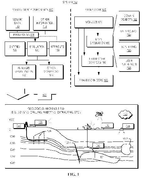
[0024] FIG. 1 illustrates an example of a system 100 that includes various
management
components 110 to manage various aspects of a geologic environment 150 (e.g.,
an environment
that includes a sedimentary basin, a reservoir 151, one or more faults 153-1,
one or more
geobodies 153-2, etc.). For example, the management components 110 may allow
for direct or
indirect management of sensing, drilling, injecting, extracting, etc., with
respect to the geologic
environment 150. In turn, further information about the geologic environment
150 may become
available as feedback 160 (e.g., optionally as input to one or more of the
management
components 110).
CA 02956951 2017-01-31
WO 2016/019302 PCT/US2015/043223
[0025] In the example of FIG. 1, the management components 110 include a
seismic data
component 112, an additional information component 114 (e.g., well/logging
data), a processing
component 116, a simulation component 120, an attribute component 130, an
analysis/visualization component 142 and a workflow component 144. In
operation, seismic
data and other information provided per the components 112 and 114 may be
input to the
simulation component 120.
[0026] In an example embodiment, the simulation component 120 may rely on
entities 122.
Entities 122 may include earth entities or geological objects such as wells,
surfaces, bodies,
reservoirs, etc. In the system 100, the entities 122 may include virtual
representations of actual
physical entities that are reconstructed for purposes of simulation. The
entities 122 may include
entities based on data acquired via sensing, observation, etc. (e.g., the
seismic data 112 and other
information 114). An entity may be characterized by one or more properties
(e.g., a geometrical
pillar grid entity of an earth model may be characterized by a porosity
property). Such properties
may represent one or more measurements (e.g., acquired data), calculations,
etc.
[0027] In an example embodiment, the simulation component 120 may operate in
conjunction
with a software framework such as an object-based framework. In such a
framework, entities
may include entities based on pre-defined classes to facilitate modeling and
simulation. A
commercially available example of an object-based framework is the MICROSOFT
.NET
framework (Redmond, Washington), which provides a set of extensible object
classes. In the
.NET framework, an object class encapsulates a module of reusable code and
associated data
structures. Object classes may be used to instantiate object instances for use
in by a program,
script, etc. For example, borehole classes may define objects for representing
boreholes based
on well data.
[0028] In the example of FIG. 1, the simulation component 120 may process
information to
conform to one or more attributes specified by the attribute component 130,
which may include a
library of attributes. Such processing may occur prior to input to the
simulation component 120
(e.g., consider the processing component 116). As an example, the simulation
component 120
may perform operations on input information based on one or more attributes
specified by the
attribute component 130. In an example embodiment, the simulation component
120 may
construct one or more models of the geologic environment 150, which may be
relied on to
simulate behavior of the geologic environment 150 (e.g., responsive to one or
more acts, whether
6
CA 02956951 2017-01-31
WO 2016/019302 PCT/US2015/043223
natural or artificial). In the example of FIG. 1, the analysis/visualization
component 142 may
allow for interaction with a model or model-based results (e.g., simulation
results, etc.). As an
example, output from the simulation component 120 may be input to one or more
other
workflows, as indicated by a workflow component 144.
[0029] As an example, the simulation component 120 may include one or more
features of a
simulator such as the ECLIPSETM reservoir simulator (Schlumberger Limited,
Houston Texas),
the INTERSECTTm reservoir simulator (Schlumberger Limited, Houston Texas),
etc. As an
example, a simulation component, a simulator, etc. may include features to
implement one or
more meshless techniques (e.g., to solve one or more equations, etc.). As an
example, a reservoir
or reservoirs may be simulated with respect to one or more enhanced recovery
techniques (e.g.,
consider a thermal process such as SAGD, etc.).
[0030] In an example embodiment, the management components 110 may include
features of a
commercially available framework such as the PETREL seismic to simulation
software
framework (Schlumberger Limited, Houston, Texas). The PETREL framework
provides
components that allow for optimization of exploration and development
operations. The
PETREL framework includes seismic to simulation software components that may
output
information for use in increasing reservoir performance, for example, by
improving asset team
productivity. Through use of such a framework, various professionals (e.g.,
geophysicists,
geologists, and reservoir engineers) may develop collaborative workflows and
integrate
operations to streamline processes. Such a framework may be considered an
application and
may be considered a data-driven application (e.g., where data is input for
purposes of modeling,
simulating, etc.).
[0031] In an example embodiment, various aspects of the management components
110 may
include add-ons or plug-ins that operate according to specifications of a
framework environment.
For example, a commercially available framework environment marketed as the
OCEAN
framework environment (Schlumberger Limited, Houston, Texas) allows for
integration of add-
ons (or plug-ins) into a PETREL framework workflow. The OCEAN framework
environment
leverages .NET tools (Microsoft Corporation, Redmond, Washington) and offers
stable, user-
friendly interfaces for efficient development. In an example embodiment,
various components
may be implemented as add-ons (or plug-ins) that conform to and operate
according to
7
CA 02956951 2017-01-31
WO 2016/019302 PCT/US2015/043223
specifications of a framework environment (e.g., according to application
programming interface
(API) specifications, etc.).
[0032] FIG. 1 also shows an example of a framework 170 that includes a model
simulation
layer 180 along with a framework services layer 190, a framework core layer
195 and a modules
layer 175. The framework 170 may include the commercially available OCEAN
framework
where the model simulation layer 180 is the commercially available PETREL
model-centric
software package that hosts OCEAN framework applications. In an example
embodiment, the
PETREL software may be considered a data-driven application. The PETREL
software may
include a framework for model building and visualization.
[0033] As an example, a framework may include features for implementing one or
more mesh
generation techniques. For example, a framework may include an input component
for receipt of
information from interpretation of seismic data, one or more attributes based
at least in part on
seismic data, log data, image data, etc. Such a framework may include a mesh
generation
component that processes input information, optionally in conjunction with
other information, to
generate a mesh.
[0034] In the example of FIG. 1, the model simulation layer 180 may provide
domain objects
182, act as a data source 184, provide for rendering 186 and provide for
various user interfaces
188. Rendering 186 may provide a graphical environment in which applications
may display
their data while the user interfaces 188 may provide a common look and feel
for application user
interface components.
[0035] As an example, the domain objects 182 may include entity objects,
property objects and
optionally other objects. Entity objects may be used to geometrically
represent wells, surfaces,
bodies, reservoirs, etc., while property objects may be used to provide
property values as well as
data versions and display parameters. For example, an entity object may
represent a well where
a property object provides log information as well as version information and
display
information (e.g., to display the well as part of a model).
[0036] In the example of FIG. 1, data may be stored in one or more data
sources (or data
stores, generally physical data storage devices), which may be at the same or
different physical
sites and accessible via one or more networks. The model simulation layer 180
may be
configured to model projects. As such, a particular project may be stored
where stored project
information may include inputs, models, results and cases. Thus, upon
completion of a modeling
8
CA 02956951 2017-01-31
WO 2016/019302 PCT/US2015/043223
session, a user may store a project. At a later time, the project may be
accessed and restored
using the model simulation layer 180, which may recreate instances of the
relevant domain
objects.
[0037] In the example of FIG. 1, the geologic environment 150 may include
layers (e.g.,
stratification) that include a reservoir 151 and one or more other features
such as the fault 153-1,
the geobody 153-2, etc. As an example, the geologic environment 150 may be
outfitted with any
of a variety of sensors, detectors, actuators, etc. For example, equipment 152
may include
communication circuitry to receive and to transmit information with respect to
one or more
networks 155. Such information may include information associated with
downhole equipment
154, which may be equipment to acquire information, to assist with resource
recovery, etc.
Other equipment 156 may be located remote from a well site and include
sensing, detecting,
emitting or other circuitry. Such equipment may include storage and
communication circuitry to
store and to communicate data, instructions, etc. As an example, one or more
satellites may be
provided for purposes of communications, data acquisition, etc. For example,
FIG. 1 shows a
satellite in communication with the network 155 that may be configured for
communications,
noting that the satellite may include circuitry for imagery (e.g., spatial,
spectral, temporal,
radiometric, etc.).
[0038] FIG. 1 also shows the geologic environment 150 as optionally including
equipment 157
and 158 associated with a well that includes a substantially horizontal
portion that may intersect
with one or more fractures 159. For example, consider a well in a shale
formation that may
include natural fractures, artificial fractures (e.g., hydraulic fractures) or
a combination of natural
and artificial fractures. As an example, a well may be drilled for a reservoir
that is laterally
extensive. In such an example, lateral variations in properties, stresses,
etc. may exist where an
assessment of such variations may assist with planning, operations, etc. to
develop a laterally
extensive reservoir (e.g., via fracturing, injecting, extracting, etc.). As an
example, the
equipment 157 and/or 158 may include components, a system, systems, etc. for
fracturing,
seismic sensing, analysis of seismic data, assessment of one or more
fractures, etc.
[0039] As mentioned, the system 100 may be used to perform one or more
workflows. A
workflow may be a process that includes a number of worksteps. A workstep may
operate on
data, for example, to create new data, to update existing data, etc. As an
example, a may operate
on one or more inputs and create one or more results, for example, based on
one or more
9
CA 02956951 2017-01-31
WO 2016/019302 PCT/US2015/043223
algorithms. As an example, a system may include a workflow editor for
creation, editing,
executing, etc. of a workflow. In such an example, the workflow editor may
provide for
selection of one or more pre-defined worksteps, one or more customized
worksteps, etc. As an
example, a workflow may be a workflow implementable in the PETREL software,
for example,
that operates on seismic data, seismic attribute(s), etc. As an example, a
workflow may be a
process implementable in the OCEAN framework. As an example, a workflow may
include
one or more worksteps that access a module such as a plug-in (e.g., external
executable code,
etc.).
[0040] As described above, the system 100 may be used to simulate or model a
geologic
environment 150 and/or a reservoir 151. In embodiments, the system 100 may be
used in field
development planning. In embodiments, the system 100 may be used to simulate
or model a
hydrocarbon field ("field"). In embodiments, the system 100 may use a multi-
point well
connection ("MPWC") method to simulate or model the field. In embodiments, the
system 100
may use the MPWC method to simulate or model fluid flow in subterranean
hydrocarbon
reservoirs of the field. In embodiments, the system 100 may use simulated or
modeled fluid flow
in planning and implementing wells in the field.
[0041] As described herein, a well cell may be indicate a grid cell with one
or more well
perforations acting as fluid sources or sinks and mathematically representing
coupling contacts
between the reservoir grid model and the well model. As described herein,
multi-point well
connection ("MPWC") may indicate a connection between a well and a number of
grid cells in
its (topological or functional) vicinity. As described herein, MPWC may also
be referred to as
multi-connection. The presence of MPWC may indicate (but not necessitate) a
support flow
across the well cell faces. As described herein, support flow may indicate
artifact flow between
a well cell and its neighbors, balancing the difference between a more
rigorous flow description
and its discrete approximation. Support flow may provide additional degrees of
freedom for
"breaking the symmetry" of the local pressure field. Support flow may channel
any solution
asymmetry from the well cell model out to the adjacent cells, causing a
corresponding distortion
of the pressure profile outside the cell. As described herein, MPWC method or
("MPWCM")
may include a mathematical method for describing and evaluating the
well¨reservoir coupling by
means of multi-connections and support flow.
CA 02956951 2017-01-31
WO 2016/019302 PCT/US2015/043223
[0042] The flow of multi-phase fluid through permeable rock may be
mathematically
described in terms of nonlinear partial differential equations (PDEs), which
may be solved by
applying numerical techniques, such as the finite volume method (FVM). The
reservoir domain
may be discretized into a grid of cells, each having its own rock and fluid
properties. Unknown
pressure, temperature, and fluid composition distributions may be approximated
by cell-wise
constant functions of space, evolving in time along finite timesteps, thus
converting the PDEs
into a large set of nonlinear algebraic equations to be solved iteratively.
The main force acting
on the reservoir fluid may come from production and injection wells, which
represent sinks and
sources in the material balance equation for each cell containing well
connections. The
perforations of the production and injection wells may mathematically
represent coupling
contacts between the two major models: the reservoir model of fluid flow
through porous media
and the well model of fluid flow through pipes. The well-to-reservoir coupling
of the two
models may be given by the equation:
(2,7 = C (PI Pw) =
(1)
where Q, may be the fluid flow-rate through the well-to-cell connection, Pi
may be the reservoir
pressure in the coupling cell i, Pw may be the wellbore (bottom-hole flowing)
pressure at some
reference well depth, and C may be the coupling coefficient, otherwise known
as the well index
or well connection transmissibility factor (when the fluid mobility is set to
1). The coefficient C
may be referred to as the productivity/injectivity index, and may combine the
connection
transmissibility (also known as well index, in case of wells with single
connections) and the fluid
mobility. The value of C may reflect the cell¨well geometry and local rock
properties.
[0043] C may be based on a quantity termed the equivalent radius of a well
block. The
equivalent radius may be one method for selecting some representative value
for Pi from a radial
pressure profile logarithmically proportional to the distance from the flowing
well. Another
approach may be based on a real averaging of the pressure profile; the
difference may be a factor
of 1.7 in the selected distance from the well. The interpretation of Pi may be
governed by two
factors: (1) taking a single value for the cell pressure from a (highly) non-
uniform distribution
around the well may be considered an upscaling process; (2) the coupling
equation (Eq. 1) may
need additional information that would provide a local reference for a more
accurate description.
[0044] The model described above may involve a number of assumptions:
stabilized flow in
the well cell, single-phase fluid, undistorted radial fluid flow, regular
geometries, vertical well
11
CA 02956951 2017-01-31
WO 2016/019302 PCT/US2015/043223
perforated across the entire permeable layer, homogeneous/isotropic rock
properties, and no
interference from neighboring wells. A few of these assumptions may be
relaxed: non-square
grids and anisotropic permeability, off-center wells and multiple wells in the
cell, and multiple
cells with flowing wells. All of these models may use the concept of
equivalent radius and may
tune the expression for C so as to adapt it to the more general cases. Varying
the magnitude of C,
however, may not fully capture the spatial asymmetry in the pressure
distortions.
[0045] Equation (1) may be a generic form of well-to-reservoir coupling
equations, including
"classical Peaceman", "projected Peaceman", "Stanford semi-analytical
approach" and others.
The focus of all these existing approaches may be on the coefficient C,
attempting to improve its
validity by lumping more and more non-uniformities from around the well
connection into its
value via complicated expressions. For example, the classical Peaceman formula
may include
anisotropy in the rock permeability of cell i. This changes the magnitude of C
by means of a
non-trivial expression involving square roots and a logarithm, however the
final effect of this
coupling equation has no directional impact on the cells outside cell i
because the vector (or
tensor) information may be lost in the single-point reservoir pressure
description in terms of the
scalar term CPL.
[0046] In embodiments, the MPWC method, for example, utilized by system 100,
may modify
Equation (1) by extending the direct communication between the well and the
well's physically
connected cell further to other cells not necessarily containing the well's
perforations. In
embodiments, the other cells may be any cells in the reservoir grid. In some
embodiments, for
example, the other cells may include the cells closest to the well connection,
e.g., the cells
directly attached to the faces of the well cell. In some embodiments, for
example, the other cells
may include cells indirectly attached to the faces of the well cell. The MPWC
may remove the
assumptions, described above, from the mathematical model by describing each
well-to-reservoir
connection in terms of a set of general formulae expressing a multi-point
representation of
reservoir pressure in which the individual coefficients capture any non-
uniformity in geometry
and rock properties around a well perforation, as well as any influence from
the surrounding
wells.
[0047] In embodiments, the MPWC method may not require any upscaling, but may
still
reflect all asymmetries in cell geometry (skewed and unstructured-grid cells),
well geometry
(slanted and curved wells, off-center and multiple wells), connection geometry
(partial and
12
CA 02956951 2017-01-31
WO 2016/019302 PCT/US2015/043223
multiple perforations, hydraulic fractures), local rock properties
(heterogeneity and anisotropy),
and external sources (nearby wells and aquifers). Figure 2 illustrates some
examples of
asymmetries in a field. The MPWC method may combine attributes of the field by
capturing the
true geometry of the coupling cell and its well perforations, internal
anisotropy and external
heterogeneity of the local rock properties, and the effect of pressure
gradients in the vicinity of
the cell, such as those caused by nearby wells. The MPWC method may be based
on a new form
of the coupling equation (Eq. 1) that may represent a boundary-integral
solution of the local
problem of single-phase fluid flow inside the well cell containing well
perforations and bounded
by its neighboring cells. In the context of FVM, the boundary conditions may
correspond to cell
pressures and inter-cell flow rates at any given time during the model
evaluation. The boundary
element method (BEM), applied to the local problem, may use cell-wise constant
FVM
quantities and may provide analytically accurate solutions at both steady and
pseudo-steady
states in the well cell (while the rest of the reservoir is at the transient
regime). The MPWC
method may propagate solution asymmetry across the faces of the coupling cell
based on the
multi-point approach. Extension to fully transient flow regimes within the
well-connection cell
(e.g., to model low-permeability high-viscosity scenarios) may be determined.
[0048] In embodiments, two MPWC models may be used in the MPWC method. One of
the
two formulations may propagate internal asymmetry (such as irregular well/cell
geometry, etc.)
outside the well-connection cell, at the additional expense of a new inter-
cell quantity (called
support flow) to be solved for. Both MPWC models may be implemented by means
of a
boundary-integral technique applied to a local flow problem within the well
cell, giving the
models their high sensitivity to geometry.
Multi-Point Approach
[0049] Consider a well that may be located exactly between two adjacent grid
cells with
identical shapes and rock properties. It may be concluded that the well
affects both cells equally.
Consider moving the well slightly into one of the cells. Although the well may
be just a
millimeter from the other cell, it may numerically lose its direct
communication with it due to the
discrete nature of the cell-wise function space. The cell containing the well,
"well cell", may
communicate with it directly via Eq. 1, while the other cell may be affected
by the well indirectly
via inter-cell flow across the shared face. In an attempt to emulate a direct
communication, the
transmissibility between the two cells may have to be increased greatly for
the case of the well so
13
CA 02956951 2017-01-31
WO 2016/019302 PCT/US2015/043223
close to the shared face. Such a change in transmissibility, to accommodate
the near-face well,
may represent a deviation from the original static model and may redefine the
relation between
the two cells.
[0050] In an extension of the example, consider three neighboring cells in a
row, perhaps as
part of a 1D-model grid. The three corresponding cell pressures may form a
vector basis for an
interpolation formula estimating pressure at any given point within the three
cells. For a well
located anywhere in the central cell, the interpolation formula may improve
the well-to-cell
coupling equation by replacing its single-point description by a (higher-
order) multi-point
description, involving pressures from more than one cell. As a result, the
well may formally
communicate (through the flow of fluid) with all the three cells directly ¨
without changing other
properties, such as the inter-cell transmissibility.
[0051] Instead of smoothing the pressure profile around the well by replacing
the cell-wise
constant function by its higher-order interpolation, the introduction of more
"pressure points"
into the coupling equation may be achieved locally within the well cell. The
interpolation
approach, mentioned previously, may effectively represent downscaling,
associated with non-
uniqueness in the choice of the basis functions and thus an uncertain outcome.
A solution of the
local flow problem, see the Boundary Integral Formulation section below, may
be a method of
coupling the well-perforation pressure, Pw, and flow rate, Qw, with the
pressure Pi of the well
cell i = 0 and of its n neighbors i > 0:
(2)
/ =0
Cs is a flow contribution from any distributed or simulated internal sources.
[0052] Eq. 2 may encapsulate the fact that flow between the well perforation
and the well cell
may not be isolated, as in Eq. 1, but depends on external factors, such as
presence of nearby
wells, reflected in the discrete pressure profile around the well cell.
Moreover, each coefficient
associated with the particular "outer cell" (i > 0) pressure may capture the
local geometry and
rock properties (including both heterogeneity and anisotropy) between the
outer cell and the well
cell. If, for example, the well perforation w is closer to cell 1 than to cell
2, or the permeability
in cell 1 is higher than in cell 2, it is expected that C1 > C2; i.e., cell 1
may have a larger
influence on the Qw vs. Pw relationship than cell 2. (This conclusion may be
valid for a highly
14
CA 02956951 2017-01-31
WO 2016/019302 PCT/US2015/043223
conductive well cell; in case of a less conductive cell, the relation among
coefficients CL in Eq. 2
may vary.)
[0053] If C1 > C2, does the well also affect cell 1 more than cell 2? In other
words, if the well
perforation is closer to cell 1 than to cell 2, would P1 show a larger change
from a uniform
profile than P2? The answer may be no, not for the case of Eq. 2. This is
because Eq. 2 enters
the overall solution process as part of the material balance equation intended
to solve the
unknown Po; the coupling equation may be associated with the well cell and
cannot be used for
the same well in cell 1. When P1 is being solved (e.g., its corresponding
equation being added to
the global system), Eq. 2 for the well in cell 0 may be ignored, and hence the
well's effect may
be felt only through the regular inter-cell flow rate. Another way of looking
at this issue may be
described as follows. Coefficients Ci>0 with different magnitudes may
propagate outer
asymmetries into the well cell and may influence the well coupling all
differently. The well cell
pressure Pc, may be adjusted accordingly, and the corresponding flow rates to
outer cells then
may reflect this change. The flow rates may be linear functions of Pi>0 ¨ Pc,
and therefore
maintain the same ratio, as in the symmetric case. Eq. 2 may enable outer
asymmetry to affect
the local flow, but may not propagate local asymmetry outside the well cell,
similar to Eq. 1.
This may be addressed by introducing the concept of "support flow"; the
coupling equation then
becomes:
(3)
i=0 i=i
[0054] The support flow, Si, may be an auxiliary quantity representing an
artifact flow
between the well cell and its neighbors, balancing the discrepancy between a
more rigorous
local-flow description and its discrete inter-cell approximation. D may be a
support flow
coefficient, which may a dimensionless term. Support flow may channel solution
asymmetry
from the well cell model out to the adjacent cells, causing a corresponding
distortion in their
pressure profile. At the same time, the support flow may provide additional
degrees of freedom
necessary for "breaking the symmetry" of the near-well pressure field.
[0055] The support flow may be similar to the steering flow in MPFA schemes,
but may play a
different role in this context. It may introduce additional unknown variables,
at most n per a
well cell (note: some cell faces may be neglected based on certain criteria;
this needs to be
further investigated), which may be the "price to pay" for the extra accuracy
provided.
CA 02956951 2017-01-31
WO 2016/019302 PCT/US2015/043223
Compared to a local grid refinement (LGR), say 3 x3 x3 in a cuboid cell, 6
unknown Si's may not
be that costly, especially when the analytical accuracy of the local flow
solution (introduced in
the next section) exceeds that of the LGR. Moreover, LGRs may require much
smaller timesteps
due to finer spatial scales.
[0056] Eqs. 2 and 3 extend the well-to-cell coupling description from a single-
cell model to a
multi-cell model. The scalar limitation of a single-point connection (Eq. 1)
may be removed in
Eqs. 2 and 3 as a consequence of the vector character of MPWC, which may
propagate near-well
positional and directional asymmetry from outer cells into the well cell (Eq.
2) or both ways (Eq.
3).
Boundary Integral Formulation
[0057] A solution of a local single-phase fluid flow problem inside one FVM
cell of arbitrary
shape, containing one or more (say rn) active well perforations of any
geometry and distribution,
and possibly belonging to more wells may be determined as discussed below. Let
the domain of
the well cell i = 0 be denoted as fl and its entire boundary F = an be
composed of n faces Fi
adjoining the outer FVM cells i > 0 to cell 0, plus in points/curves/surfaces
Fõ, representing the
well perforations. The pressure values P. of these cells or perforations, and
the corresponding
flow rates Q. across F., may provide boundary conditions (BCs) for the local
problem. If any of
the outer cells are inactive or missing, the appropriate global boundary
condition may be applied
instead. Conservation of the fluid mass (or moles, depending on the density p)
may yield the
material balance equation
V = q + 1 a(p(P)
= o , in fl , at t > t',
(4)
p at
where is the rock porosity, t denotes time and t' is its initial value. The
macroscopic fluid
velocity q in the rock pore-space may follow Darcy's law:
q = ¨K = Vp , K = ¨u1 .
(5)
[0058] As discussed herein, p and P are referred to as "pressures", but may
also be termed
pressure potentials, as they implicitly include the gravitational term pgAz,
where p and q
represent the real-space quantities, while P and Q are their discrete-space
counterparts.
16
CA 02956951 2017-01-31
WO 2016/019302 PCT/US2015/043223
[0059] In Eq. 5, the permeability tensor k may be assumed to be diagonal
(e.g., the Cartesian
coordinates in fl are already aligned with the principal axes of the
permeability tensor). Property
pt may be the dynamic fluid viscosity and the unit conversion factor u1 is
specified in Table 1.
[0060] Table 1
Symbol SI Value Field Value
0.00852702 0.00632829
U2 U1 0.00112712
U3 1.0 U3 = u1/u2
[0061] Under an assumption of "small pressure gradients", the fluid density
may be eliminated
from Eq. 4 by means of another property, ct, capturing the total
compressibility of the fluid¨rock
system; Eqs. 4 and 5 are then combined in the pressure-diffusion equation
ap
v = (K = Vp) ¨ Oct ¨ = 0 , in ,Q, , at t > t' .
(6)
- at
[0062] Eq. 6 may be solved for the prescribed initial and boundary conditions
defined next.
Both Pi and Qi may be given, whereas only Pw or Qw may be given while the
other value is to be
found:
p = p' , in ,Q, , at t = t' ,
(7a)
p = f (Põ Pi+) , on F, , at t t', for outer cell i = 1, ,n ,
(7b)
P = Pw on Fw at t > t', for well perforation w = 1,
... ,m ,
= on F, , at t t', for outer cell
i = 1, n ,
(7c)
q = Qw/I FW I , on Fw at t t', for well perforation w = 1,
=== m =
Here, q may represent the normal component of the velocity vector, q E q =ii,
where ñ may be
the unit outward vector normal to the boundary F*, the area of which may be
expressed as I F. I
Generally, II may vary along a curved boundary; however, in the case of FVM
cells with mostly
flat faces, it may be taken as constant on each Fi, which somewhat simplifies
the solution
procedure. (Note: the Solved Examples section illustrates how the variation of
ii is handled on
circular/cylindrical wellbore surfaces Fw .) Another convenient fact dictated
by the FVM may be
the uniformity of Pi and Qi over each Fi, leading to further simplifications
in the BEM-based
formulation. At the moment, let the function f (Pi, P1 ) be simply Pi; its
extension to linearly
interpolated cell pressures may be discussed below in the Examples section.
[0063] This may pose a question about the continuity of p over F. When Pi
generally differs
between two boundary segments Fi, the pressure field may become multivalued in
the
corresponding corner and the fluid velocity approaches infinity there. This
kind of singularity
17
CA 02956951 2017-01-31
WO 2016/019302 PCT/US2015/043223
may appear all over the FVM grid due to its cell-wise constant function space.
As described
herein, the discontinuous pressure field may cause no difficulty; the internal
field p(x E Si) may
not be explicitly required, and may not be computed.
[0064] When handling nonlinear or spatially varying material properties and
distributed
internal sources, the boundary-only character of BEM may encounter a domain
integral that
cannot be directly converted to a boundary integral, but may not appear for
the local problem
defined in Eqs. 6 and 7, as all material properties are spatially constant in
fl, due to the FVM
treatment of its cell properties. At the same time, all internal sources
(specifically the well
perforations) may be excluded from the domain by interpreting them as part of
the boundary F.
[0065] At this point, before the solution of the local flow problem may be
detailed, the
difference equation generated by the FVM-based solver for each cell of the
reservoir grid may be
introduced. Here, the focus may be on the well cell 0:
fl 711
(21 + Qw + 1 AGXPV)
___________________________________ = 0, in no ,at t = t' + Lt.
(8)
p At
t=1 w=1
[0066] Eq. 8 may be a discrete form of Eq. 4, approximating the material
balance over cell 0 of
volume V at time t' + At, where At is the timestep. The multi-phase form of
the equation may
include additional parameters, such as phase saturation, formation volume
factor, etc., and it may
be intended target for the MPWC method, except that the method itself may
treat the fluid
locally (in the well cell) as a homogeneous mixture of phases.
[0067] The volumetric rate of fluid flow from cell 0 into cell i, across their
shared face Fi, may
be a function of their pressure difference, inter-cell transmissibility Ti,
and fluid mobility Mi. An
extra term may be added, in accordance with Eq. 3, and may be the support flow
Si (note: the
permeability ratio Ki and the uniform support flow Ui may be ignored: Ki := 1,
Ui := 0):
Q, = ¨T,M,(P,¨ P0) + K,S, + U.
(9)
[0068] This discrete form of Darcy's law may be used as the Neumann boundary
condition in
Eq. 7c for the local flow problem. Both Pi and Qi may be known at any time t
as a result of
solving n Eqs. 8 of their respective cells. In a defined problem, only one of
the two well-
perforation quantities (i.e., either Pw or Qw) may prescribed at any given
time t as part of some
user-specified constraints involving group, well, and completion controls. The
two cases are
discussed later.
Boundary Integral Equation.
18
CA 02956951 2017-01-31
WO 2016/019302 PCT/US2015/043223
[0069] A starting point of the boundary element method, previously also known
as the
boundary integral equation, may be a general form of the boundary integral
equation (BIE). The
BIE may represent an alternative formulation of the problem originally defined
in terms of PDE
and its associated conditions; it may be derived from Green's second identity,
involving free-
space Green's functions as its kernels. For the problem defined in Eqs. 6 and
7, the kernels may
be functions of space, rock and fluid properties, and optionally of time for
fully transient
regimes; their specific details may be deferred to section Time Dependence. To
generalize, Eq. 6
may be rewritten as
L(p) = ¨a,
(10)
and its adjoint equation, defining the corresponding free-space Green's
function G, may be
expressed as
(11)
The self-adjoint linear differential operator L may satisfy the general form
of Green's second
identity:
f[p L(G) ¨ G L(p)] dco = f K = [p VG ¨G V IA = ri dy. .
(12)
El r
[0070] Both Eq. 10, where o- is any source in fl, and Eq. 11, where the Dirac
delta S represents
a point source at x', may be substituted into Eq. 12, together with the
definition of kernel F E F =
ii associated with G:
F = ¨K = VG .
(13)
Upon applying the sifting property of the delta function and rearranging, Eq.
12 becomes
c(x') p(x') = f [p(x) F(x-x') ¨ q(x) G(x- x')] dy + f a (x) G(x- x') dco .
(14)
r El
[0071] Eq. 14 is the boundary integral equation which may be used to solve Eq.
10 subject to
the prescribed boundary conditions. It may relate pressure at any given point
x' to the boundary
values p and q (first integral, x E F) and to internal source density o-
(second integral, x E SO; the
latter is discussed in the section Time Dependence. The "contact coefficient"
c may have a
value of unity inside the domain (x' E 11) and less than one, 0 < c < 1, on
the boundary (x' E
F); it may reflect the boundary geometry in the x' vicinity. Point x' may be
even excluded from
the closure fl U F completely by setting c = 0.
19
CA 02956951 2017-01-31
WO 2016/019302 PCT/US2015/043223
[0072] There may be a direct link between the BIE, represented by Eq. 14, and
the MPWC,
described by Eqs. 2 and 3: the latter may be particular cases of the former.
Although the BIE
may be just one of a number of ways how to generate the coupling equations for
MPWCs (e.g.,
others may include LGRs), it may be more accurate and efficient.
[0073] In embodiments, in an FVM model, a grid of cells may be traversed at
each solution
time t and a set of (nonlinear) algebraic equations may be generated for every
primary solution
quantity in the cell. In a stencil of n cells attached to the central cell 0,
the unknown cell
pressure Pc, may be found by evaluating Eq. 8 (with Eq. 9) and adding it to
the global residual
vector (e.g., all Eqs. 8) and Jacobian matrix (e.g., the gradient of all Eqs.
8 with respect to all
unknowns), which are then solved for all the unknowns. If cell 0 contains any
well connections,
the corresponding flow rates Q, may need to be added to the material balance,
Eq. 8. The two
possible constraints are: (1) value of Q, may be specified and may be directly
used in Eq. 8; (2)
value of /3, may be specified and hence the corresponding Q, in Eq. 8 may be
expressed
indirectly by means of a coupling equation. In embodiments, the relationship
between /3 and
Q, based on the MPWC method (e.g., Eq. 2 or 3) may be implemented via Eq. 14.
[0074] For example, the following analysis may assume a single well
perforation in cell 0. For
case (1), mentioned in the previous paragraph, there may be no need to
generate Eq. 2, whereas n
instances of Eq. 3 may be required to find the n unknown support flow
variables Si, as discussed
later. For case (2), Eq. 2 may be formed once, while Eq. 3 may lead to n + 1
instances: 1 for the
unknown Q, and n for the unknown Si 's.
[0075] To generate one Eq. 2 or 3 for a well perforation of known pressure /3
(e.g., derived
from the prescribed bottomhole pressure using head calculations in the
wellbore), point x' may
be positioned on the boundary Fõõ representing the perforation's contact with
rock, and Eq. 14
may be evaluated by carrying out the particular integrations. All quantities
in Eq. 14 may be
known, except the missing value of Q, introduced through q on F. Specifically,
c, F and G
may be computed from the geometry, while p and q may be prescribed on U F = F
\ F by
means of Eqs. 7b¨c. Both types of boundary conditions on Fi may contain cell
pressures Pi
(note: q indirectly via Eq. 9) which may be solved by FVM and therefore may
need to be treated
as unknowns when Jacobian entries are collected from Eq. 14. The final step,
after all CL
coefficients are computed, may be to cast Eq. 14 into the form of Eq. 2 or 3
and insert the
resulting Q, into Eq. 8. In other words, the FVM equation may be used for
finding the well-cell
CA 02956951 2017-01-31
WO 2016/019302 PCT/US2015/043223
pressure Pc, (and other solution quantities), but its well-inflow term may
capture complex near-
well features causing the local flow to deviate from a pattern assumed in Eq.
1.
[0076] In some embodiments, the procedure may be extended to multiple
perforations in the
well cell (i.e., rn > 1) with the exception that even the case (1) constraint
now requires its own
Eq. 14 [note: if the case (1) constraint may treated as an internal source
rather than a boundary
condition, the extra Eq. 14 may not needed]. This is because only one from the
pair of boundary
conditions on Fw may be prescribed, whereas the other may not be known. As
multiple
perforations communicate with each other, values of both Qw and Pw may be
available in Eq. 14
to uniquely define mutual influences between the sources. Eqs. 2 and 3 thus
need to be generated
from Eq. 14 for every perforation w, by positioning point x' on the
corresponding Fw, and the
resulting flow rates Qw may then be added to Eq. 8. Furthermore, each of these
equations must
be appended to the global solution system (residual and Jacobian) to support
the unknown
constraint, the value of which is to be found. Considering Eq. 3, for example,
the set of rn
equations to solve for the [unknown(Pw, Qw)]õT=1 vector may be written as
A=Qw =B=P-C=Pw+D=S+E.
(15)
[0077] Since the support flow variables S may represent yet another set of
unknowns,
additional n equations (Eq. 3) may be required in the global system. The
matrices and (column)
vectors in Eq. 15 then have the following sizes: A = [rn+n, rn], Qw = [in], B
= [rn+n, n+1],
P = [n+1], C = [rn+n,in], Pw = [in], D = [rn+n, n], S = [n] and E = [rn+n].
Unlike the
equations to determine the missing well constraints, which may also applied in
Eq. 8 to replace
Qw, the S-related equations may not be used anywhere else.
[0078] While generating Eqs. 3 to solve for S, point x' in Eq. 14 may be
positioned near or on
the well-cell face i associated with the unknown Si. In general, point x' in
the BIE may represent
a fictitious point source whose influence on all parts of the boundary (or
boundary elements)
may be expressed in terms of kernels G and F. Kernel G captures the distance
between x' and the
integration point x, while F also reflects the local boundary orientation
towards x'. Therefore,
moving point x' in Eq. 14 to the vicinity of a particular feature in fl U F
may also move the BIE' s
focus on that feature. Each such new equation may be linearly independent from
the others due
to the strong spatial nonlinearities in the kernel functions (assuming non-
degenerate x'
distribution). In practical terms, this may enable generating a well-
conditioned, diagonally
dominant (due to singularities in BIE) set of algebraic equations for
determining any unknown
21
CA 02956951 2017-01-31
WO 2016/019302 PCT/US2015/043223
boundary quantities, such as p or q. In the case of support flow, the same
approach may help to
find Si such that its value compensates for the error in Qi (see Eq. 9) caused
by the approximate
FVM description of the inter-cell flow rate. By positioning point x' in Eq. 14
near or on the cell
face F, the BIE may be instructed to focus on the relation between the face's
Pi and Q. As these
quantities may be given (e.g., solved elsewhere), the BIE's analytical
"expectation" of their
relationship results in adjusting the free parameter associated with the face,
i.e. the support flow
Si.
[0079] In some embodiments, for example, two adjacent FVM cells both may
contain well
perforations. When one of these cells is being processed as cell 0 while the
other supplies its Pi,
the support flow Si associated with their shared face may be adjusted
according to the BIE model
of cell 0 only. In other words, the Qi compensation via Si may not reflect
fluid sources and sinks
located within cell i. As there may only be one value of Si, balancing the
flow from both sides
of the face, the two cells may be merged while evaluating Eq. 14 for this
particular Si. The
local-flow problem domain thus may combine the two cells, fl =I U I, with
possibly
different rock and fluid properties. The so-called concept of zones may be
applied to such
sectionally heterogeneous media, while considering when the permeability-
anisotropy directions
differ in the two zones. No more than two cells may need to be merged for each
Si, even though
well perforations may appear in more or all of the outer cells. This is
because each particular Si
may be associated with the face Fi shared only by two cells: the well cell 0
and the outer cell i.
[0080] Returning to a general case of any well-cell model, three additional
conditions may be
secured to make sure that the support flow represents a correct complement to
the inter-cell flow
given by Eq. 9. Firstly, Si may be restricted by the permeability of the outer
cells, while no
support flow may be expected for completely non-conductive cells as the
extreme case. This
may be achieved by multiplying Si by the permeability ratio Ki appearing in
Eq. 9 and defined as
K, = max(K, = ri = Kg', 1) max(k,/ko , 1) for ,u, pto and k ¨> k .
(16a)
[0081] The maximum function may prevent amplification of Si for more
conductive outer
cells, as the well cell is controlling the flow. The first term in Eq. 16a may
apply generally for
anisotropic media and fluid viscosity varying strongly between cells, whereas
the second term
may assume neither of those cases and gives Ki its simplified name.
[0082] The implementation of Eq. 16a in the BIE via Eq. 9 may require care
while applying
the equations. In all instances of these equations, Ki may follow Eq. 16a,
except in one particular
22
CA 02956951 2017-01-31
WO 2016/019302 PCT/US2015/043223
instance where it may be forced to unity. This instance may be Eq. 15 to find
Si for which Ki :=
1, while, in the same equation, KJ, associated with all the other outer cells
(j # i) comes from Eq.
16a by default. The interpretation of this exception may be: Eq. 14, producing
Eq. 15 for Si, may
find the correct compensation of Qi from the well-cell's viewpoint, ignoring
the target-cell's
properties, which do not apply locally. These properties may be taken into
account later in terms
of the correct Ki (Eq. 16a), which restricts the maximum Si "suggested" by the
specially treated
Eq. 9 while forming the corresponding Eq. 15.
[0083] The second condition may be explained by considering a well with a
prescribed flow
rate. When Qv,/ is given, the material balance over the well cell may be
defined and may not be
violated. Due to the FVM-introduced pressure discontinuities at the well-cell
faces (i.e., between
Pc, and Pi on Ft), the overall support flow may become nonzero, Izi Si I 0,
and therefore may
cause an imbalance in the total flow from/into the cell: Ei Qi ¨Q, (at steady-
state, see Eq. 8).
To handle this, a compensation may be used via the following "uniform support
flow"
u, = ______________________________________ ,
(16b)
where Ai = IFi I is the face area. The idea behind Eq. 16b is to sum up the
individual support
flows in a bulk flow and then compensate for it by its complement, uniformly
distributed among
all faces according to their "conductance".
[0084] In some embodiments, to prevent any artifact fluid source caused by
excess/shortage in
the total support flow, the uniform support flow defined in Eq. 16b may be
added to Eq. 9 in all
instances, except one an instance when Eq. 15 may be generated for the
corresponding unknown
Si. In that particular case, UL may be set to zero, while the other values of
Uj, j # i, should again
use Eq. 16b. This exception may be analogous to the previously discussed Si
condition, and its
explanation is also similar: When Eq. 14 generates Eq. 15 for the unknown Si,
its target value
may not be "hindered" by any compensations that are supposed to be applied
afterwards.
[0085] The third condition that may need to be addressed is to ensure that the
support flow
does not duplicate any flows resulting from differences in outer-cell
pressures, which may be
handled strictly by the FVM-based Eq. 8. To accomplish that, any background
support flow
computed by means of Eq. 15 for all internal sources "turned off' may be
subtracted from the
support flow computed for the sources "turned on". The role of the support
flow may be to
redistribute flow from/to the internal sources to/from non-default outer
cells, as compared to the
23
CA 02956951 2017-01-31
WO 2016/019302 PCT/US2015/043223
homogeneous flow distribution imposed by Eq. 1. Although the total amount of
well
inflow/outflow may differ due to the S-induced changes in pressure, S should
clearly exclude
inter-cell flow corresponding to the pressure variation around the well cell
(and not caused by
sources in the well cell).
[0086] To implement a source-only, rather than total, support-flow
computation, the S-related
n Eqs. 15 may be applied twice with the same coefficients B and D: (1) to
compute the
background flow without any sources, and (2) to compute the net flow caused by
well-cell
sources only. In the first case, coefficients A and C may be set to zero in
Eqs. 15, effectively
removing all well flow from the equations. Such equations may be resolved
immediately, e.g.,
not necessarily as part of the global system, to obtain the values of the
background support flow
S. In the second case, the regular coefficients A and C computed from the BIE
may be used in
Eq. 15, and the unknown S-variables may be replaced by the sum of net and
background support
flow: S S + g. Hence, the "new" S-unknowns, resolved as part of the global
system, may
reflect only flow between wells and the appropriate outer cells.
[0087] In some embodiments, the unknown variables /3, and Q, for multiple
perforations in a
cell, and Si may be generalized. A possibility of an alternative formulation
may avoid the need
for introducing these unknowns and solving for them as part of the global
system. During the
time-stepping process, at each new time t = t' + At, the solution from the
previous time t' may
be fully known and thus available for any direct computations. When Eq. 8 is
being assembled
and the values of Q, are needed, any quantities in Eq. 14, which would require
additional BIEs
added to the global solution system may be taken from the solution at the
previous time level.
This may represent a mixed time-level scheme. Such an approach may eliminate
the need for
adding Eqs. 15 to the global system. Another possibility may be to keep the
implicit character of
the local-flow model, but carry out the solution of Eqs. 15 locally rather
than globally. This may
correspond to a multi-scale (or multi-grid) approach to PDE solving, where the
coarse scale may
be the FVM grid and the fine scale may be the BEM-based model of each well
cell. In that case,
Eqs. 15 may be resolved immediately when their unknowns may be needed in Eq.
8, using the
latest global solution values at time t and current Newton step (or nonlinear
solver iteration).
Further local updates may be frozen after a specified number of Newton steps
in order to allow
the global system to reach convergence. The set of Eqs. 15 may be small, only
in + n unknowns
24
CA 02956951 2017-01-31
WO 2016/019302 PCT/US2015/043223
where both numbers are of the order of ten, and therefore a direct solver may
be the preferred
choice.
[0088] In some embodiments, various techniques may be used to evaluate the
integrals in Eq.
14. Analytical expressions for simple kernels to specialized Gaussian
quadratures may be used
to deal with integrable singularities, such as the logarithmic singularity in
2D. The initial step
may be finding the boundary point x closest to x', splitting the boundary
segment/patch around
it, and if x = x', treating the integral in the Cauchy principal value sense.
In some embodiments,
several options may be used for a choice of the actual x' location on the
local boundary (FL or
Fw). There may be several options for where to position point x' on Fi,
including geometric
centroid, inter-cell connector, or "everywhere" ¨ in a double convolution
integral sense.
[0089] In some embodiments, well skin factor, s, may be an auxiliary reservoir
engineering
(RE) concept which extends existing well-to-cell coupling equations, such as
Eq. 1, to damaged
(s > 0) or stimulated (s < 0) wells by assuming a layer of rock with
permeability ks around the
well perforation, with ks < k and ks > k for the two respective cases of well
skin. Although the
MPWC-based coupling equations (Eqs. 2 and 3) may use more complex models than
Eq. 1, the
well skin may be added to them by modifying the boundary conditions /3, and
Qv,/ in Eqs. 7b¨c
by using a Robin-type BC. Dynamic, or flow-dependent, well skin may extends
the skin concept
by adding turbulent and inertial effects of high-velocity near-well flow
regimes, usually around
gas wells. Forchheimer correction may be applied to the Darcy flow Eqs. 5 and
9, generalizing
them to equations of non-Darcy fluid flow. All equations involving the flow
velocity q or rate
Q, such as Eqs. 4, 7c, 8 and 14, may be affected by the additional flow-
dependent term and lead
to extended forms of the equations derived from them, including Eqs. 6, 10, 11
and 13. These
equations may be linearized, so that the previously described solution
procedure may be
extended to non-Darcy flow regimes.
[0090] In embodiments, the boundary integral formulation may be sensitive to
the geometry of
the local domain, e.g., shape of the well cell and distribution/shapes of its
well perforations. In
embodiments, internal solutions in the domain itself may not be required ¨
only the boundary
distribution of pressures and velocities may be sought, thereby reducing the
number of
unknowns. The BIE may be a suitable tool for the MPWC representation; no
upscaling/downscaling may be involved. In Eqs. 7c, 9 and 14, no assumption may
be made
about the value of Po. As mentioned previously, Eq. 1 may need to postulate a
certain value for
CA 02956951 2017-01-31
WO 2016/019302 PCT/US2015/043223
the well-cell pressure, for example, based on the pressure equivalent radius.
In the MPWC
method, the value of Pc, may enter the model as part of the boundary
conditions for the local
problem, and those may be fully consistent with the global FVM-based
description of the
reservoir.
Time Dependence
[0091] The boundary integral equation, Eq. 14, may represent an integral
formulation of the
local flow problem defined generally by Eq. 10. The particular forms of
kernels G and F may
depend on the differential operator L; once it is specified, together with the
internal source o-, the
BIE may be evaluated to provide the coupling equation for MPWCs (Eq. 2 or 3).
Three time-
models are discussed in the following subsections, presented in the order of
their increasing time
dependence.
Steady State
[0092] Pressure diffusion in anisotropic media, with no time dependence, may
be described by
the Laplace equation (see also Eq. 10):
L(p) E V = (K = Vp) , o- = 0 .
(17)
[0093] The particular expressions for the free-space Green's functions G and F
that satisfy the
adjoint system, Eqs. 11 and 13, are listed below for both 2D and 3D domains;
see Eqs. A-4.
[0094] Two points, x and x', in a Euclidean space of two or three dimensions
may have
geometric distance
r = V (x-xt)2 + (y-yt)2 in 2D , r = V (x-xt)2 + (y-yt)2 + (z-zt)2 in 3D,
(A-1)
and "anisotropic distance"
i
R = + _____ in 2D, R = + _____ + (x-x')2i(X-X')2 (Z-
Z)2
___________________________________________________________ in 3D,
(A-2)
K, K
Y Y
in a medium described by a diagonal tensor K, see Eq. 5. Another measure to be
utilized may be
the normal component of their positional vectors' difference
= (x - xt) = ii,
(A-3)
where II is the unit outward vector normal to the local boundary: 11(x) 1 F
(x) A li = fi = 1.
[0095] The function G, which satisfies Eq. 11 where L is the Laplacian, and
the corresponding
function F, which represents a normal component of F defined in Eq. 13, may
have the following
expressions:
26
CA 02956951 2017-01-31
WO 2016/019302 PCT/US2015/043223
¨ ln R rn
G = ____________________________ , F = _______________ in 2D,
(A-4a)
271-VKõKy 271-VKõKy R2
1 rn
G = ____________________________ , F = in 3D.
(A-4b)
47 A ficKyKz R 47.1K,tKyKz R3
[0096] Similarly, function G, satisfying Eq. 11 where L is the modified
Helmholtz operator
(discussed in section Transient State), and its corresponding function F, may
be expressed, as
follows:
Kn(RVoct/At) rn VoctiAt Ki(RV Oct/At)
G = , F = _____________________________________________ in 2D,
(A-5a)
271-.\/K,cKy 27.\ I KxKy R
exp(¨RVOct/At) rn (1 + RVOctiAt) exp(¨RVOct/At)
G = __________________________ F = _________________________ in 3D.
(A-5b)
47-1-A I K,KyK, R ' 47-1-A I K,KyK, R3
[0097] In Eq. A-5a, Ko and K1 are the modified Bessel functions of second kind
and of order 0
and 1, respectively.
[0098] As a consequence of the zero internal source, the domain integral in
Eq. 14 may vanish,
leaving behind just the boundary integral to be processed.
[0099] The steady-state model may assume that the fluid flow is stabilized not
only locally in
the well cell, but also throughout the entire reservoir, and hence the
accumulation term in Eq. 8
may be omitted. This model may be suitable for testing MPWCs' sensitivity to
asymmetric
setups.
Pseudo-Steady State.
[00100] The pseudo-steady state model may assume a stabilized flow regime
within the well
cell, and a transient flow regime outside the cell (e.g., in the rest of the
reservoir). Eq. 10 may
compensate for the additional accumulation term in Eq. 8 by treating it as an
internal sink, so that
the material balance in the local flow problem is consistent with the FVM
description:
AP0
L(p) E V = (K = Vp) , a = ¨Oct¨At .
(18)
The expressions for the kernels G and F may be identical to those of the
steady-state model,
namely Eqs. A-4. However, the domain integral in Eq. 14 may be dealt with.
[00101] To avoid domain integration and restore the boundary-only character of
the BIE, the
domain integral may be converted to a boundary integral by applying the (Gauss-
Ostrogradsky)
divergence theorem. This may be possible only because o- is constant in fl and
because G, in
27
CA 02956951 2017-01-31
WO 2016/019302 PCT/US2015/043223
both 2D and 3D, may be a relatively simple function at steady state. The
conversion is given by
the formula:
f o- G do) = 1 - o- f rõ(G + a) dy , a=1(4n-VicKy)1 in2D ,
(19)
2 0 in 3D
El r
[00102] where rn is defined in Eq. A-3 and G in Eqs. A-4.
[00103] The pseudo-steady state model may cover scenarios in which the well-
cell diffusivity
K/(OctV) may be large enough for the local flow to reach a steady regime
within a fraction of
timestep At since the last change in the well control constraints. The
existing well-to-cell
coupling models represented by Eq. 1 assume stabilized flow in the well cell,
although some of
them update their coefficients frequently to approximate evolution in time.
The same may hold
for the pseudo-steady state model described here, with dynamic updates due to
the pressure
variables of the surrounding cells built directly into the MPWC coupling
formulae.
Transient State
[00104] Certain classes of problems, such as low-permeability and high-
viscosity scenarios,
may require the local flow problem to be treated as time-dependent. In that
case, the transient
pressure-diffusion equation (Eq. 6) may be converted to the integral form of
Eq. 14, and its time-
derivative term may need a special treatment. Three basic types of atp
treatments may include:
convolution in time, integral transform (e.g., Laplace transform), and time-
stepping process. The
first two approaches may avoid the domain integral, but may expect smooth
solution variation in
time. The third approach may include a domain integral, but its time-
derivative handling may be
identical to that of FVM, and may be consistent with Eq. 8. The linear
differential operator L
and the internal source o- of Eq. 10 in the time-difference form become:
P'
L(p) E V = (K = V p) ¨ (pcP, ¨ o- = (pc ¨ . (20)
t At t At
[00105] This L may be known as the modified Helmholtz operator, and its
corresponding free-
space Green's function (based on Eq. 11) may involve a modified Bessel
function in 2D, Eq. A-
5a, and an exponential function in 3D, Eq. A-5b.
[00106] The pressure p' at previous-time level t' = t ¨ At may be a function
of space, and
therefore the domain integral may not be converted to a boundary integral
(although techniques,
such as the dual-reciprocity or multiple-reciprocity BEM may provide
mechanisms for doing so).
To numerically evaluate the domain integral, the well-cell domain fl may be
tessellated into
28
CA 02956951 2017-01-31
WO 2016/019302 PCT/US2015/043223
auxiliary finite elements, and their approximation of the p' field may be
integrated over each
element using its basis functions. The auxiliary mesh/grid may not introduce
any new
unknowns; it only facilitates evaluation of the domain integral. The p'
distributions in all well
cells may be stored between timesteps. Pressure values inside the domain may
be obtained using
the same boundary integral equation, Eq. 14, as are pressure values on the
boundary, except that
the contact coefficient now represents a full contact of point x' with the
domain by setting c = 1.
[00107] Figure 3 illustrates a flowchart of a method 300 for evaluating a
hydrocarbon field
using a MPWC method. The illustrated stages of the method are examples and any
of the
illustrated stages may be removed, additional stages may be added, and the
order of the
illustrated stages may be changed.
[00108] In 302, a field may be determined for which to simulate the operation
of the field. In
some embodiments, for example, a user of the system 100 may select a field to
evaluate. In
some embodiments, for example, the system 100 may automatically select a field
for evaluation.
[00109] In 304, formation properties and fluid properties may be determined
for the field. In
some embodiments, a user may specify the formation properties and fluid
properties. In some
embodiments, the formation properties and fluid properties may be determined
by the system
100, for example, using data measured, sensed, collected, etc. by the system
100. In some
embodiments, the formation properties and fluid properties may be stored by
the system 100 and
may be retrieved by the system 100.
[00110] In some embodiment for example, the formation properties may include
rock properties
such as permeability, porosity, geometry of the rock, anisotropies in the
rock, and any other
geological properties of the field. The fluid properties may include fluid
density, composition,
pressures in the wells, and any other physical properties that describe fluids
in the field. .
[00111] In 306, the field may be divided into grid cells. In some embodiments,
for example, the
reservoir domain may be tessellated into grid cells. In some embodiments, the
grid cells may be
small segments of generally irregular geometry. In some embodiments, the grid
cells may be
assigned rock properties, for example, the formation properties determined in
304. In some
embodiments, the rock properties may vary between grid cells.
[00112] In 308, one or more wells, location of the one or more wells, and
configurations of the
one or more wells may be determined for the field. In some embodiments, the
one or more wells
may include existing wells in the field. In some embodiments, the one or more
wells may
29
CA 02956951 2017-01-31
WO 2016/019302 PCT/US2015/043223
include one or more new wells proposed for the field. In some embodiments, for
example, the
one or more wells may include injection wells. In some embodiments, for
example, the one or
more wells may include production wells.
[00113] In some embodiments, the location of the one or more wells may include
the grid cell in
which the one or more wells are located. In some embodiments, the
configuration of the one or
more wells may include the type of wells (e.g., injection or production), the
shape of the one or
more wells, the dimensions of the one or more wells, number and type of
perforations in the one
or more wells, and the like.
[00114] For example, the one or more wells may intersect any number of cells
along the well's
trajectory of arbitrary shape. In some embodiments, grid cells containing well
perforations, e.g.
well-to-reservoir connections, may represent coupling contacts between the
mathematical models
describing the well's segments and the reservoir grid.
[00115] In 310, the multi-point well connection method may be performed to
simulate
operations in the field. As described above, the formation properties, the
fluid properties, one or
more wells, location of the one or more wells, and configurations of the one
or more wells may
be utilized to simulate fluid flow within the field and to simulate operation
of the field.
[00116] In some embodiments, for example, at least one of the one or more
wells may be
selected to simulate and evaluate parameters of the at least one of the one or
more wells. In
some embodiments, the formation properties, the fluid properties, one or more
wells, location of
the one or more wells, and configurations of the one or more wells may applied
to Equation (2),
as discussed above, to simulate and evaluate parameters of the at least one of
the one or more
wells. In some embodiments, for example, the formation properties, the fluid
properties, one or
more wells, location of the one or more wells, and configurations of the one
or more wells may
applied to Equation (3), as discussed above, to simulate and evaluate
parameters of the at least
one of the one or more wells. In embodiments, for example, the MPWC method may
utilize the
boundary integral, as discussed above, to determine boundary conditions in the
grid cells. For
example, the MPWC method may utilize the boundary integral, as discussed
above, to determine
unspecified boundary conditions in the grid cells, which may not be defined in
the formation
properties, the fluid properties, one or more wells, location of the one or
more wells, and
configurations of the one or more wells
CA 02956951 2017-01-31
WO 2016/019302 PCT/US2015/043223
[00117] In embodiments, for example, the MPWC method may produce simulated
field results
311 that include the parameters of the at least one of the one or more wells
simulated by the
MPWC method. The simulated field results 311 may include fluid flow in the
formation,
pressure at the one or more wells, and fluid flow at the one or more wells,
and any other
parameters that represent operation of the one or more wells. In some
embodiments, for
example, the simulated field results may include data that represents
operation of the field at a
single point in time. In some embodiments, for example, the simulated field
results may include
data that represents operation of the field over time.
[00118] In 312, the field may be analyzed for different wells or well
configurations. In some
embodiments, for example, a different well from the one or more wells may be
selected for
evaluation. In some embodiments, for example, a location and configuration of
at least one of
the one or more wells may be modified and evaluated. In some embodiments, for
example, one
or more new wells may be added to the field and evaluated.
[00119] If the field is further analyzed, the method 300 may return to 308 and
repeat the MPWC
process for the different wells or well configurations. If analysis is
complete, the process may
proceed to 314. In 314, further analysis may be performed on the simulated
field results 311. In
some embodiments, for example, the simulated field results 311 may be
displayed for analysis by
a user. For example, the simulated field results 311 may be displayed in
different formats for
analysis by the user such as a numerical representation of the simulated field
results, a graphical
representation of the field results and the like. In some embodiments, for
example, the simulated
field results 311 for a specified time may be displayed and analyzed. In some
embodiments, for
example, the simulated field results 311 over a specified period of time may
be displayed and
analyzed. In some embodiments, for example, the simulated filed results may be
stored by the
system 100 or transmitted to other computer system. In some embodiments, for
example, the
simulate field results 311 may be used to plan installation of new wells,
operations of existing
wells, and the like.
[00120] Figure 4 illustrates an example of flow determined using the MPWC
method as
compared to Equation 1. Panel 1 illustrates pressure distribution due to an
off-center injection
well as determined by Equation (1): Th. = p2 = p3 = p4. Panel 2 illustrates
pressure distribution
due to the off-center injection well as determined by Equation (3): Pt = p2 >
p3 = p4. Panel 3
illustrates pressure distribution due to a kx> ky anisotropy in the well cell
with an injection well
31
CA 02956951 2017-01-31
WO 2016/019302 PCT/US2015/043223
in the center, as determined by Equation (1): Pt = p2 = p3 = p4. Panel 4
illustrates pressure
distribution due to a k, > ky anisotropy in the well cell with an injection
well in the center, as
determined by Equation (3): Pt = p3 > p2 = p4.
Examples
[00121] The discussion below describes four examples of the MPWC method
performed using
experiential data for a test field.
Example 1
[00122] The aim of the first example is to compare accuracy of the proposed
MPWC models
(Eqs. 2 and 3) against a published analytical solution as well as results from
a commercial
numerical simulator. During the discussion of this example, the models defined
by Eqs. 2 and 3
may be referred to as the "S-free" and "S-based" models, respectively. The
problem to solve and
the test field may be a steady flow of liquid through a square-shaped
reservoir, surrounded by a
constant-pressure aquifer, towards a single producing vertical well in the
center. In this example,
the geometry and the rock/fluid properties may be defined as: L = 100 ft, A =
L2, h = 10 ft, r =
0.5 ft, k = 5 md,
= 0.5, ct = 10-5 1/psi, u = 0.5 cP, B = 1 RB/STB, PL = 1,000 psi, and
Q, = 100 STB/D. In this example, the flowing wellbore pressure may be
described by the
formula:
p = p 1 in ( 16A 141.2/3,4õ
(21)
2 kh
where y = 1.781 is the exponential of Euler's constant and CA = 30.88 is the
shape factor for a
well in the center of a square reservoir. Applying the data and evaluating,
the wellbore pressure
value may be found as: /3 = 339.05 psi.
[00123] Next, the boundary-integral approach based on Eq. 14 may be performed.
The
boundary integral equation (Eq. 14) applied to a simple two-dimensional,
steady-state problem of
a square reservoir with a single producing well in the center and surrounded
by a constant-
pressure aquifer, may be expressed as a zero sum of two integrals:
0 = + .
(B-1)
[00124] The zero value on the left-hand side may come from c(x') = 0 for the
point x'
positioned in the center of a circle representing the well boundary F. This
"no contact" case,
representing a line-source approximation of a cylindrical source in 3D, may be
an interpretation
of the BIE and the evaluation of integral I,, may be as follows:
32
CA 02956951 2017-01-31
WO 2016/019302 PCT/US2015/043223
27rr,
/w,w = (Pw¨Ir(wR2 qw -27lnKR) dy = pw + qwrw ln(r,,,VK)
2K
(B-2)
0
[00125] The kernels G and F in Eq. 14 may replaced by their 2D steady-state
specializations
(Eq. A-4a) applied to isotropic media (K K) and using r = rw and R = rwK-2 for
their
distances defined in Eqs. A-1 and A-2, respectively. The distance vector r = x
¨ x' may be a
constant radial direction perpendicular to the boundary Fw but oriented
towards the domain fl;
hence, its outward-normal component is negative: rn = ¨rw. Although the
direction of ñ varies
with y, rn itself may be independent of y, which may be a simplification
arising from circular
and spherical Fw 's in 2D and 3D, respectively. If the active well perforation
surface has a more
complex curvature, the normal distance rn may be expressed as a function of y
and the integral
may be evaluated numerically. Alternatively, the curved boundary Fw may be
split into flat
boundary elements which would provide analytical expressions for integrals
with simple kernels,
such as those in Eqs. A-4.
[00126] The second integral in Eq. B-1 may make use of the rotational symmetry
when point x
moves along the outer square boundary and point x' still resides in the middle
of the domain.
Given the simplification that the aquifer pressure pi may be uniform around
the reservoir, the
eight identical boundary integrals over the edge-halves may be written as
L/2
= 81( L/2 ¨1nR
1312n-KR2 '71 2n-K )dY = (B-3)
In this case, however, the distance between points x and x' may be dependent
on y,
r = V(L/2)2 + (L/2 ¨ y)2 , R = r /VT( ,
(B-4)
while the outward-normal component stays constant, rn = L/2. Eq. B-3 may be
evaluated
analytically as
Ltln[L2/(2K)] ¨ 2)
= p, + q, _______ = (B-5)
WI n-K
The normal fluxes qw and qi may be assigned from the prescribed well flow rate
Qw according
to the following formulae,
Qw13 ¨(2w13
qw = ____________________________ U3 , q, = __ U3 ,
(B-6)
2n-rwh Lh
33
CA 02956951 2017-01-31
WO 2016/019302 PCT/US2015/043223
where the unit conversion factor u3 is listed in Table 1. Upon applying the
geometric
dimensions and rock/fluid properties from the first solved example into Eqs. B-
2, B-5, and B-6,
with p,, = 13*, and solving Eq. B-1 for Pw, its value may be found to be
331.09 psi. .
[00127] The requirement of spatially constant qi (but not necessarily pi, as
demonstrated in the
third solved example) built into the proposed MPWC method may originate from
the intention to
keep the number of newly introduced unknowns low. This may provide a
straightforward
coupling of the BEM-based local-flow model with the FVM-based reservoir-flow
model by
means of outer-cell pressures Pi and inter-cell flow rates Qi (see Eq. 9). The
required values of
transmissibility and mobility may calculated for the examples as
= k1h1u2 , mi = ¨ ,
(B-7)
Bit
assuming two-dimensional domain, single-phase fluid, and constant viscosity.
[00128] When the S-based model is considered, the additional Eqs. 15 may be
required for
determining the four support flow rates Si may be generated from Eq. 14
adapted to the square-
shaped domain, as follows:
= + 11,1 + 211,1 1+11,1 2. (B-8)
The cells may be counted sequentially around the well cell, and their indices
may naturally cycle
when reaching the extrema. Point x' may be positioned on face/edge i, which is
reflected in the
half-domain contact on the left-hand side of Eq. B-8. A number of discrete
choices may be
available for the actual x' location, whereas a continuously varying location
leads to double
convolutions:
= ¨ f f [p F(x-x') ¨ G(x-x')] dy dy' , x' E , x E .
(B-9)
fi fõ
The following may the particular forms of such integrals for the problem under
investigation:
rw [2 ln[L2/(2K)] + it ¨ 4)
= qw ______________
4K
L [ ln(L2/K) ¨ 3]
= q, ____________________________________
47K
(B-10)
ln(4) + it L [2 ln(2L2/K) + it ¨ 6]
k1+1 = pi _________________ 87 + qi
87K
it ¨ ln(4) L [1n(L2/K) + it ¨ 3]
1.1,1+2 = Pi ____________ qi =
47K
34
CA 02956951 2017-01-31
WO 2016/019302 PCT/US2015/043223
[00129] For illustration purposes, one numerically evaluated Eq. B-8 (for i =
1) may be given
as:
3.46571 P0 - 1.21385 P1 - 0.713848 P2 - 0.824166 P3 - 0.713848 P4
+ 6.33338 S1 + 7.93178 S2 + 8.55142 S3 + 7.93178 S4 + 7.65905 Qw = 0 . (B-11)
Eq. B-1 in the S-based model may have the following coefficients,
3.45307 P0 - 2.45307 P, - Pw + 30.6362 S, + 0.969969 Qw = 0 ,
(B-12)
where Pi and Si apply to each face/edge due to the symmetry (i.e., their
coefficients are sums of
the four equal contributions). Setting Si := 0 may convert Eq. B-12 directly
from the S-based
model to the S-free model.
[00130] Using the above process the value of Pw = 331.09 psi may be
determined. The same Pw
value may be obtained when the square domain is treated as a well cell and
gets surrounded by
eight outer cells of the same geometry, four of which adjoining its
faces/edges i = 1, ...,4. The
cell pressures Pi may be assigned the aquifer pressure value of 1,000 psi and
may represent
Dirichlet boundary conditions for the local problem, see Eq. 7b. The Neumann
boundary
conditions (Eq. 7c) may be supplied to cell 0 by means of inter-cell flow
rates, described by Eq.
9 in an S-based model or with Si := 0 in an S-free model, in the form of Eq. B-
6 for this
particular problem setup. Eq. 9 may introduce a new unknown into the
mathematical model, not
appearing in Eqs. B-1-6, namely the well-cell pressure Po. As mentioned
previously, the
MPWC method may avoid making any assumption on the relation between Po, Pw and
Qw,
unlike the existing approaches based on Eq. 1 (e.g., using the concept of
equivalent radius). The
MPWC method may couple the BEM-based model of the well cell (Eq. 14 yielding
Eq. B-1), to
find the unknown Pw, with the FVM-based model of the well-cell's neighborhood
(represented
by Eq. 8), to find the unknown Po. Eq. 8 may be applied to the symmetric
problem under
consideration simplifies (with Eq. B-7) to
Qw = 4 TM(P, - P0) = 0.450848(P, - P0) ,
(22)
and therefore may give Po = 778.2 psi. The outcome of the BEM-based local
model may not
affect the value of Po in this case at all, because Qw is prescribed whereas
Pw is to be found. If
the well control was swapped (e.g., Pw prescribed and Qw to be found), the
value of Po resulting
from Eq. 8 may depend on the outcome of the well-cell model as a consequence
of adding Eq. 14
to Eq. 8 through the corresponding Q. In either case, no new unknowns may be
introduced in
CA 02956951 2017-01-31
WO 2016/019302 PCT/US2015/043223
the S-free model for a single active well perforation in the well cell as
described above for
multiple perforations.
[00131] In the S-based model, up to n new unknown support flow rates Si may be
added to the
local well-cell model in order to redistribute the otherwise uniform well flow
in accordance with
various (inner and outer) asymmetries. The S-based model may not produce
results that differ
than those of the S-free model. The concrete forms of two Eqs. 15 for this
model may be
detailed in Eqs. B-11 and B-12, which, for the same value of Po as stated
before, yield the
solution: Si = 0.0912 STB/D and P = 333.89 psi. The support flow may help to
improve the
accuracy of p by adjusting the inter-cell flow rates Q.
[00132] Closer inspection of the overall material balance in the well cell,
however, may indicate
that the symmetric nonzero Si value leads to a difference between the
prescribed well flow rate,
Q, = 100 STB/D, and the inter-cell flow rates, -Ei Qi = 99.6352 STB/D. This
may be
corrected by involving the uniform support flow rate Ui, defined in Eq. 16b,
according to the
procedure described along with the equation. When the uniform support flow
rate is expressed
as UL = Si and inserted into Eq. 9 (with the described exceptions), the new
value of the
support flow rate may become Si = ¨Ui = 0.4428 STB/D. At the same time, the
updated values
of Po, Põ, and Q, may return to the above-mentioned values computed by the S-
free model. This
occurs because the support flow rate may be practically eliminated from all Qi
's for this
symmetric problem setup. In non-symmetric cases, where the resulting Si
differs from face to
face, the preservation of material balance through UL may leave non-zero net
support flows in the
corresponding Qi's, in agreement with the local asymmetries.
Example 2 - Time-Dependent Flow
[00133] The parameters from Example 1 may be used to test the pseudo-steady
state description
of transient fluid flow by means of Eqs. 18 and 19. As such, the wellbore
pressure over time
may be determined. In some embodiments, the wellbore pressure over time may be
plotted to
determine when the wellbore pressure reaches steady state. For this particular
example, the true
stabilization time may appear to be roughly 0.5 day, and the pseudo-steady
state approximation
behind Eq. 18 may be acceptable for timesteps of one day and more. If the
transient effects in
the well cell dominate the simulation timesteps, the fully transient MPWC
model represented by
Eq. 20 may be used.
Example 3 - Outer Asymmetry Acting on a Well Cell.
36
CA 02956951 2017-01-31
WO 2016/019302 PCT/US2015/043223
[00134] The Examples 1 and 2 illustrates the MPWC method when applied to a
symmetric
problem setup. Example 3 may introduce an external asymmetry (e.g., not caused
by the well
cell itself), by means of a linear pressure gradient between two constant-
pressure boundaries at
different pressure potentials, 100 psi and 1,900 psi. The overall geometry and
rock/fluid
properties may be the same as in Example 1 and 2, but the well in the middle
may be converted
into an observation well by zeroing its Qõ while computing its unknown põõ
which may be
expected to be 1,000 psi ¨ the average of the edge pressures. Another
observation well may be
positioned into local cell {19, 19} of a Cartesian LGR inside global cell {2,
2} that is to be
tested.
[00135] When tested, the wellbore pressure in the center well may be
determined to be 1,000
psi. Both S-free and S-based MPWC models may determine results for the corner-
well
bottomhole pressure: Põ, = 664.346 psi. In another test, the Dirichlet
boundary condition on the
well-cell faces may be improved. The function f (Pi, Pi+) in Eq. 7b may be
fixed to a constant
value of Pi. The outer pressure field may be linear, but the well-cell
boundary may treat it as
constant. The choice of f may not limited to constant functions and a boundary-
value
description may be used in terms of a linear function involving pressures of
the outer cells
sharing edges in 3D or corners in 2D with the current outer cell i:
L ¨ y P, + P,_ y P, + P, 1
f (Pi, Pi+) = _________________ 2 , y E [0, L] . ________________________
(23)
L 2
[00136] Eq. 23 may be specific to the problem in question, and the usual
cycling of indices may
apply. Upon modifying the MPWC method by implementing Eq. 23 into their BIEs,
both the 5-
free model and the S-based model predict the corner wellbore pressure to be
Põ, = 657.143 psi, as
expected. The linear function may be more representative of pressure gradients
surrounding the
well cell in general and may be preferred to the default constant f. Other
schemes may be
designed, even MPFA-type schemes involving nine points in the MPWC rather than
five in 2D.
[00137] An explanation may be due regarding the role of support flow in the S-
based solution of
Example 3. No fluid may be flowing into/from the observation wells and hence
Si may stay zero,
but that is not what happens. The outer pressure gradient may be reflected on
the well-cell faces
and may be interpreted by the BIE as a non-zero flux through the domain.
Although the inter-
cell flow rate Qi may represents the flux correctly, pressure discontinuities
between cells i and
cell 0 may lead to non-zero values of Si, although their overall balance is
zero: Eisi = 0. This
37
CA 02956951 2017-01-31
WO 2016/019302 PCT/US2015/043223
may be a different issue from the one discussed in the first example. This may
be addressed by
computing a source-only support flow Si by subtracting the background support
flow gi from the
original total S. In Example 3, gi = gi and hence Si = O. The S-based model
may behave
similar to the S-free model after the background flow is eliminated from the
former.
Example 4 - Local Asymmetry Acting on Outer Cells.
[00138] In Example 1-3, both MPWC models produce the same results, while the S-
free model
may have no additional unknowns and no associated issues to deal with. Example
4 may
illustrate how the S-based model may propagate the local asymmetry outside the
well cell.
Example 4 may use the same domain geometry and rock/fluid properties as in the
previous
examples, as well as the producing well from the first example moved to a
location of the corner
well in the third example. In this example, the main extension may come in
terms of another
layer of FVM cells around the domain, resulting in a 5x5 global grid with the
well-cell in the
middle. The sixteen outermost cells may be kept at constant pressure of 1,000
psi, whilst their
eight inner neighbors may be free to respond to the well-induced pressure
changes in the single
innermost cell.
[00139] For both symmetric and asymmetric well locations inside a 21x21
Cartesian LGR, the
center and corner wells reside in local cells {11, 11} and {19, 19},
respectively. For the the 5-
based MPWC method (with f = Pi in Eq. 7b and a double-integration via Eq. B-
9), the wellbore
pressures as 220 and 240 psi may be determined for the two respective wells.
The calculated
support flow rates may be ¨23.166 and 22.693 STB/D (with UL = 0.2365) for the
cell faces
closest to and furthest from the corner well, respectively. The S-based model,
may reproduce the
shift in the outer pressure profile, observed around the LGR. This may show
the model's
capability to broadcast a local asymmetry in the well cell (e.g., due to off-
center well location,
irregular cell shape, etc.) out to the adjacent cells through the additional
support-flow variables.
[00140] In some embodiments, the methods of the present disclosure may be
executed by one or
more computing systems. Figure 5 illustrates an example of such a computing
system 500, in
accordance with some embodiments. The computing system 500 may include a
computer or
computer system 501A, which may be an individual computer system 501A or an
arrangement
of distributed computer systems. The computer system 501A includes one or more
analysis
modules 502 that are configured to perform various tasks according to some
embodiments, such
as one or more methods disclosed herein. To perform these various tasks, the
analysis module
38
CA 02956951 2017-01-31
WO 2016/019302 PCT/US2015/043223
502 executes independently, or in coordination with, one or more processors
504, which is (or
are) connected to one or more storage media 506. The processor(s) 504 is (or
are) also
connected to a network interface 507 to allow the computer system 501A to
communicate over a
data network 509 with one or more additional computer systems and/or computing
systems, such
as 501B, 501C, and/or 501D (note that computer systems 501B, 501C and/or 501D
may or may
not share the same architecture as computer system 501A, and may be located in
different
physical locations, e.g., computer systems 501A and 501B may be located in a
processing
facility, while in communication with one or more computer systems such as
501C and/or 501D
that are located in one or more data centers, and/or located in varying
countries on different
continents).
[00141] A processor may include a microprocessor, microcontroller, processor
module or
subsystem, programmable integrated circuit, programmable gate array, or
another control or
computing device.
[00142] The storage media 506 may be implemented as one or more computer-
readable or
machine-readable storage media. Note that while in the example embodiment of
Figure 5
storage media 506 is depicted as within computer system 501A, in some
embodiments, storage
media 506 may be distributed within and/or across multiple internal and/or
external enclosures of
computing system 501A and/or additional computing systems. Storage media 506
may include
one or more different forms of memory including semiconductor memory devices
such as
dynamic or static random access memories (DRAMs or SRAMs), erasable and
programmable
read-only memories (EPROMs), electrically erasable and programmable read-only
memories
(EEPROMs) and flash memories, magnetic disks such as fixed, floppy and
removable disks,
other magnetic media including tape, optical media such as compact disks (CDs)
or digital video
disks (DVDs), BLURAY disks, or other types of optical storage, or other types
of storage
devices. Note that the instructions discussed above may be provided on one
computer-readable
or machine-readable storage medium, or alternatively, may be provided on
multiple computer-
readable or machine-readable storage media distributed in a large system
having possibly plural
nodes. Such computer-readable or machine-readable storage medium or media is
(are)
considered to be part of an article (or article of manufacture). An article or
article of
manufacture may refer to any manufactured single component or multiple
components. The
storage medium or media may be located either in the machine running the
machine-readable
39
CA 02956951 2017-01-31
WO 2016/019302 PCT/US2015/043223
instructions, or located at a remote site from which machine-readable
instructions may be
downloaded over a network for execution.
[00143] In some embodiments, computing system 500 contains field analysis
module 508. In
the example of computing system 500, computer system 501A includes the
drilling volume
module 508. In some embodiments, a field analysis module may be used to
perform some
aspects of one or more embodiments of the method 300 disclosed herein. In
alternate
embodiments, a plurality of field analysis modules may be used to perform some
aspects of
method 300 herein.
[00144] It should be appreciated that computing system 500 is merely one
example of a
computing system, and that computing system 500 may have more or fewer
components than
shown, may combine additional components not depicted in the example
embodiment of Figure
5, and/or computing system 500 may have a different configuration or
arrangement of the
components depicted in Figure 5. The various components shown in Figure 5 may
be
implemented in hardware, software, or a combination of both hardware and
software, including
one or more signal processing and/or application specific integrated circuits.
[00145] Further, the steps in the processing methods described herein may be
implemented by
running one or more functional modules in information processing apparatus
such as general
purpose processors or application specific chips, such as ASICs, FPGAs, PLDs,
or other
appropriate devices. These modules, combinations of these modules, and/or
their combination
with general hardware are included within the scope of the present disclosure.
[00146] For reference, the list below provides a summary of notation used in
equations
discussion herein.
A, B = MPWC coefficients in Eq. 15
= = formation volume factor, RB/STB [rm3/sm3]
ct = total compressibility, L.t2/m, 1/psi [1/bar]
= = well connection coefficient, L4.t/m
= support flow coefficient, dimensionless
= boundary condition function; default: f =
= = (flux) free-space Green's function
= acceleration due to gravity, 0.006944 ft2.psi/lbm
= = (potential) free-space Green's function
CA 02956951 2017-01-31
WO 2016/019302
PCT/US2015/043223
I ki ¨ boundary integral (Eq. 14) over Ft with x' on Fk
h = formation thickness (or height), L, ft [m]
k = absolute rock permeability, L2, md
K = kill, conductivity, L3.t/m, md/cP
KN = modified Bessel function of 2nd kind, of order N
L = length, L, ft [m]
m = number of well perforations in well cell
M = fluid mobility, L.t/m, 1/cP
n = number of outer cells surrounding well cell
II = unit outward normal to boundary F
p = pressure potential, m/L.t2, psi [bar]
P = cell pressure potential, m/L.t2, psi [bar]
q = macroscopic fluid velocity, Lit, ft/D [mid]
Q = volumetric flow rate, L3/t, STB/D [sm3/d]
r = radius or Euclidean distance, L, ft [m]
R = "anisotropic" distance, (m/L.t) -2
s = well skin factor, dimensionless
S = support flow rate, L3/t, STB/D [sm3/d]
t = time, t, D [d]
T = transmissibility, L3, RB.cP/D.psi [rm3.cP/d.bar]
u = unit conversion factor
U = uniform support flow rate, L3/t, STB/D [sm3/d]
V = volume, L3, ft3 [m3]
x, y, z = Cartesian coordinate, L, ft [m]
Greek and Other Symbols
y = parameter of boundary F
F = boundary (of local flow problem)
S = Dirac's delta function
A = difference
L = linear differential operator
K = permeability ratio, dimensionless
41
CA 02956951 2017-01-31
WO 2016/019302 PCT/US2015/043223
ii = dynamic fluid viscosity, m/L.t, cP
P = mass fluid density, m/L3, lbm/ft3 [kg/m3]
o- = internal source
0 = effective rock porosity, dimensionless
co = parameter of domain fl
fl = domain (of local flow problem)
Subscripts and Superscripts
0 = well cell
i = cell (index); outer cell: i > 0
n = normal component
s = well skin
w = well perforation
,
= specified value
* = "all types"
[00147] The foregoing description, for purpose of explanation, has been
described with
reference to specific embodiments. However, the illustrative discussions above
are not intended
to be exhaustive or limiting to the precise forms disclosed. Many
modifications and variations
are possible in view of the above teachings. Moreover, the order in which the
elements of the
methods described herein are illustrate and described may be re-arranged,
and/or two or more
elements may occur simultaneously. The embodiments were chosen and described
in order to
best explain the principals of the disclosure and its practical applications,
to thereby enable
others skilled in the art to best utilize the disclosed embodiments and
various embodiments with
various modifications as are suited to the particular use contemplated.
42