Note : Les descriptions sont présentées dans la langue officielle dans laquelle elles ont été soumises.
CA 03034807 2019-02-22
WO 2018/080460 PCT/US2016/058692
ESTIMATING INTERVAL ANISOTROPY PARAMETER FOR PRE¨STACK DEPTH
MIGRATION USING A LEAST¨SQUARES METHOD
BACKGROUND
[0001] Certain earth formations exhibit a property called
"anisotropy", where the velocity of acoustic waves polarized in
one direction may be somewhat different than the velocity of
acoustic waves polarized in a different direction within the
same earth formation. Anisotropy may arise from intrinsic
structural properties, such as grain alignment, crystallization,
aligned fractures, or from unequal stresses within the
formation.
[0002] In the presence of seismic
anisotropy,
conventional primary wave (P-wave) data processing based on
the assumption of isotropy typically results in errors in depth
images and interpretations. A transversely isotropic model with
a vertical symmetry axis (VII) represents one of the most
effective approximations to the subsurface formations and has
been widely applied to anisotropic pre-stack depth migration
(PSDM) over the past several decades; knowledge of a vertical
velocity and two Thomsen parameters is essential to produce
accurate depth images of P-wave data.
[0003] For VII media, one critical step in correcting for
anisotropy in PSDM is the estimation of reliable interval
anisotropy parameters in depth domain from P-wave data combined
-1-
CA 03034807 2019-02-22
WO 2018/080460 PCT/US2016/058692
with borehole and other non-seismic information. Despite recent
successes, anisotropy parameter estimation in depth domain
remains a highly challenging and unsolved problem. In recent
years, many approaches to invert for interval VII anisotropy,
specifically the interval anellipticity parameter ri, have been
developed in reflection seismology. Most of these methods were
implemented in the time domain using Dix-type inversion, and a
time-to-depth conversion based on 1D approximation was then
applied to obtain an interval anellipticity parameter for
anisotropic PSDM. The interval anellipticity parameter can be
refined in the depth-migrated domain using advanced reflection
tomography or wave-equation migration velocity analysis for
complex geological environments.
BRIEF DESCRIPTION
[0004] Reference is now made to the following descriptions
taken in conjunction with the accompanying drawings, in which:
[0005] FIG. 1 is a schematic diagram showing a cross-
sectional view of an illustrative environment with seismic
sources, seismic receivers, a wellbore and a computing system,
according to certain embodiments of the present disclosure;
[0006] FIG. 2 is a block diagram of an apparatus for
estimating interval anisotropy parameter according to certain
embodiments of the present disclosure;
-2-
CA 03034807 2019-02-22
WO 2018/080460 PCT/US2016/058692
[0007]
FIG. 3 is a flow diagram for a method of estimating
interval anisotropy parameter; and
[0008]
FIG. 4A, FIG. 4B, FIG. 4C, and FIG. 4D illustrate
numerical test results for comparing the disclosed least-squares
method for estimating interval anellipticity parameters with a
traditional method.
DETAILED DESCRIPTION
[0009]
The Dix-type equation noted above analytically inverts
effective anellipticity parameter for interval anellipticity
parameter as a function of vertical travel time. It is realized
herein that traditional Dix-type inversion is known to be an
ill-posed inverse problem, even under the assumption of
horizontally layered geological environments.
For a thin
interval, small errors in the effective anellipticity parameters
could have a dramatic effect on the estimated interval
anellipticity parameter.
It is desirable to find a stable and
inexpensive estimate of interval anisotropy parameter at the
early stages of parameter inversion for seismic anisotropy.
[0010]
Accordingly, the disclosure provides an apparatus and
methods that accurately estimate the interval annellipticity
parameter in the depth domain.
[0011]
This disclosure provides a more accurate Dix-type
equation and its explicit inverse in the depth domain that
-3-
CA 03034807 2019-02-22
WO 2018/080460 PCT/US2016/058692
directly inverts effective anellipticity parameter for interval
anellipticity parameter as a function of depth. A robust and
effective least-squares method is developed to invert directly
the effective values of anellipticity parameter for interval
values in depth domain, i.e., the input data and output data for
the proposed Dix-type inversion are both in depth domain. In
addition, a prior knowledge of interval normal moveout (NMO)
velocities obtained from an isotropic tomography using the near-
offset P-wave data helps stabilize and constrain the solution of
the proposed least-squares method. Moreover, this disclosure
inverts the interval anellipticity parameter in the depth domain
which presents the data processor with a stable initial
parameter for anisotropic depth migration. Thus, this disclosure
establishes a more robust approach than simply estimating
starting parameters for anisotropic velocity model building.
[0012] FIG. 1 is a schematic diagram showing a cross-
sectional view of an illustrative environment 100 with seismic
sources 102, seismic receivers at the surface 104, a wellbore
106, a computing system 108, and seismic receivers in the
wellbore 114 according to certain illustrative embodiments of
the present disclosure. An energy (e.g. acoustic wave)110 from
one or more of the seismic sources 102 at or near the surface
travels through subterranean formation 112, reflects off of
various subterranean formations or geological features, and is
-4-
CA 03034807 2019-02-22
WO 2018/080460 PCT/US2016/058692
subsequently collected as seismic data at the surface using the
surface receivers 104 or within the wellbore 106 using wellbore
receivers 114. For certain embodiments, the subterranean
formation 112 can be anisotropic, i.e., propagation speed of
acoustic waves may depend on the direction in which the acoustic
wave propagates.
[0013] The computing system 108 may be configured to acquire
seismic data associated with the subterranean formation 112 from
the surface receivers 104 or the wellbore receivers 114, and
perform estimation of anisotropy parameters of the subterranean
formation 112 as disclosed herein and discussed in further
detail below. For example, the seismic data can include P-wave
data from which a measured effective annellipticity parameter
can be extracted and an estimated interval annellipticity
parameter can be determined in depth domain.
[0014] In one or more embodiments, the computing system 108
may be further configured to utilize the estimated anisotropy
parameters of the subterranean formation 112 and perform
anisotropy PSDM and anisotropy migration velocity analysis (MVA)
providing coherent depth images and an accurate seismic data
volume associated with the subterranean formation 112. For some
embodiments, the obtained coherent depth images and the accurate
seismic data volume of the subterranean formation 112 obtained
by taking into account anisotropy parameters of the subterranean
-5-
CA 03034807 2019-02-22
WO 2018/080460 PCT/US2016/058692
formation 112 may be utilized in real time for drilling of the
wellbore 106. In general, the presented method for estimation of
anisotropy parameters of subterranean formations may be applied
for obtaining more coherent depth images of hydrocarbon
reservoirs in the subterranean formation leading to more
efficient drilling of wellbores and increased hydrocarbon
production.
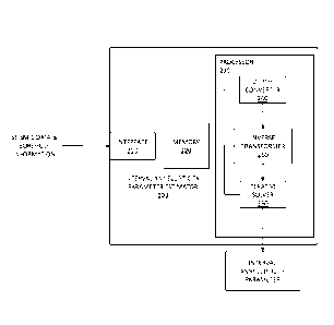
[0015]
FIG. 2 illustrates a block diagram of an interval
annellipticity parameter estimator 200 that estimates an
interval annellipticity parameter according to the principles of
the disclosure. The interval annellipticity parameter estimator
200 can be implemented on a computer, such as the computing
system 108 illustrated in FIG. 1. The interval annellipticity
parameter estimator 200 includes an interface 210, a memory 220,
and a processor 230. The interface 210, the memory 220 and the
processor 230 can be connected together via conventional means.
[0016]
The interface 210 is configured to receive seismic
data, borehole information and other non-seismic data for the
annellipticity parameter estimator 200.
The interface 210 can
be a conventional interface that is used to receive and transmit
data. The interface 210 can include multiple ports, terminals or
connectors for receiving or transmitting the data.
The ports,
terminals or connectors may be conventional receptacles for
communicating data via a communications network.
The seismic
-6-
CA 03034807 2019-02-22
WO 2018/080460 PCT/US2016/058692
data includes P-wave data, from which measured effective
annellipticity parameter can be extracted. In addition, a prior
knowledge of interval NMO velocities can be obtained from an
isotropic tomography using the near-offset P-wave data. The
borehole information may be used to extract vertical
information, such as vertical velocity and vertical travel time.
[0017]
The memory 220 may be a conventional memory that is
constructed to store data and computer programs. The memory 220
includes a data reservoir configured to store data needed for
the annellipticity parameter estimator 200. The memory 220 may
store operating instructions to direct the operation of the
processor 230 when initiated thereby.
The operating
instructions may correspond to algorithms that provide the
functionality of the operating schemes disclosed herein.
For
example, the operating instructions may correspond to the
algorithm or algorithms that convert a Dix-type equation into
depth domain.
In one embodiment, the memory 220 or at least a
portion thereof is a non-volatile memory.
[0018] The processor 230 is configured to determine an
interval annellipticity parameter. The processor 230 includes a
depth converter 240, an inverse transformer 250 and an iterative
solver 260.
In one embodiment, the memory 220 or a portion
thereof can be part of the processor 230.
-7-
CA 03034807 2019-02-22
WO 2018/080460 PCT/US2016/058692
[0019]
The depth convertor 240 is configured to convert a
function of effective anellipticity parameter into depth domain
based on the vertical information extracted from the borehole
information. In one embodiment, the function of effective
anellipticity parameter in depth domain is a Dix-type equation
that states the linear relationship between an effective
anellipticity parameter and an interval anellipticity parameter.
[0020] The effective anellipticity parameter in the depth
domain is approximately given by the following Dix-type equation:
1
___________________________ +8)70.1-#4:- .
= 8 to(2,1/õ4õ0.0 11.:pogl 1 Eq. 1
[0021]
From equation 1, to is the vertical travel time
calculation from the vertical velocity obtained from the
borehole information, Vnmo is the interval normal moveout
velocity, Vp0 is the vertical velocity and z and
are the depth,
respectively. Next, the inverse transformer 250 is configured to
set up a rearranged Dix-type equation in depth domain as a
least-squares fitting problem based on the measured effective
anellipticity parameter obtained from the P-wave seismic data.
For example, the effective anellipticity parameter can be
estimated by analyzing the residual moveout on isotropic depth-
migrated common image gathered after the application of an
isotropic tomography using P-wave seismic data.
-8-
CA 03034807 2019-02-22
WO 2018/080460 PCT/US2016/058692
[0022] In order to invert for the interval anellipticity
parameter ri, Eq. 1 can be rearranged to:
_r4
8/Az) ____ "in __ 817(Adc: .
Eq. 2
[0023] In one embodiment, for stratified VII media composed
of regularly spaced horizontal layers, equation 2 can be set up
in a least-squares fitting goal:
d - WFmi-e Eq. 3
where d is the known data computed from the measured effective
anellipticity parameter, m is the model containing interval
anellipticity parameter to be inverted for, e is an error
vector, F is the smoothing operator like causal integration that
is scaled by the term V4,,mo/Vp0 in equation 2, and W is the data
weighting function computed from the term 1/toVinino in equation 2.
[0024] The inverse problem (Eq. 3) can be solved in a least-
squares sense by taking the model that minimizes an objective
function itr, defined by equation 4 below for the covariance
matrices C, and Cm:
Illgtt);;: WFINITC;01 - Fm) F ni"Cjlek.
Eq. 4
[0025] The positive-definite matrix C., plays the role of the
variance of the error vector e. The second term of * defines a
stabilizing functional on the model space. In practice, an
inverse covariance matrix Ce-1 relates to the data residual
-9-
CA 03034807 2019-02-22
WO 2018/080460 PCT/US2016/058692
weighting operator multiplied by its adjoint and an inverse
covariance matrix Cm-1- relates to the roughening operator, for
example, second-difference operator, multiplied by its adjoint.
[0026] The iterative solver 260 is configured to employ
iterative methods to solve the least-squares fitting problem
(Eq. 4) for an anisotropy model containing an interval
anellipticity parameter. The number of iterations needed depends
on the initial model and the final goal. Applicable iterative
methods include conjugate-gradients, Gaussian-Newton, LSQR
(Least squares with QR factorization), etc.
[0027] In one embodiment, the iterative solver 260 employs a
method of conjugate-gradients (CG) for minimizing the objective
function itr. The gradient in the CG method is the gradient of the
objective function * and is determined by taking the derivative
of the objective function * with respect to the model.
[0028] For certain embodiments, the iterative solver 260 is
configured to apply a prior knowledge of interval normal moveout
velocity obtained from an isotropic tomography as constraints of
the anisotropy model. Additional constraints contribute to the
fast convergence in inversion process: preconditioning by
parameterizing model with a smooth, bounded function and
regularization with geological constraints. The iterative solver
260 is configured to output an anisotropy model which contains
the interval anellipticity parameter.
-10-
CA 03034807 2019-02-22
WO 2018/080460 PCT/US2016/058692
[0029] Now turning to Fig. 3, illustrated is a flowchart for
illustrating a method 300 for estimating an interval
anellipticity parameter. The method 300 can be performed by a
computer program product that corresponds to an algorithm that
estimates an interval anellipticity parameter as disclosed
herein. The method 300 may be carried out by an apparatus such
as the interval anellipticity estimator 200 described in Fig. 2.
The method begins in a step 305.
[0030] In a step 310, seismic data and borehole information
are received. The received seismic data can be preprocessed for
extracting measured effective anellipticity parameter, vertical
information such as vertical velocity and vertical travel time,
and a prior knowledge of interval normal moveout velocity.
[0031] In a step 320, a Dix-type equation that states the
linear relationship between an effective anellipticity parameter
and an interval anellipticity parameter is converted into depth
domain. A rearranged Dix-type equation in depth domain is set up
as a least-squares fitting problem based on the measured
effective anellipticity parameter in a step 330. A step 340
employs an iterative method to solve the least-squares fitting
problem for an anisotropy model containing interval
anellipticity parameter. Applicable iterative methods may
include conjugate-gradients, Gaussian-Newton and LSQR. A prior
knowledge of interval normal moveout velocity obtained from an
-11-
CA 03034807 2019-02-22
WO 2018/080460 PCT/US2016/058692
isotropic tomography may be applied as constraints of the
anisotropy model. In step 350, an anisotropy model containing
interval anellipticity parameter is obtained from the solution
of the least-squares fitting problem. The method 300 ends in a
step 360.
[0032] FIG. 4A, FIG. 4B, FIG. 4C, and FIG. 4D illustrate
numerical test results for comparing the disclosed least-squares
method for estimating interval anellipticity parameters with a
traditional method. The test results are based on a horizontally
layered VII model with blocky interval anellipticity parameters
and P-wave vertical velocity linearly increasing with depth,
i.e., 171,0(z)= 3.0(1+0.083z). The minimum vertical velocity is
3.0 km/s at the surface of the model and the maximum vertical
velocity is 4.0 km/s at the depth of 4.0 km of the model. The
synthetic effective anellipticity parameters are calculated
using Eq. 1 and are then added with uniform distributed random
noise. The x-axis in each figure is the interval anellipticity
parameter eta and the y-axis is depth.
[0033] FIG. 4A shows the input data of effective
anellipticity parameters with random noise used to invert for
the interval anellipticity parameters. In FIG. 4B, 4C and 4D,
solid line 1 represents the true model, dashed line 2
represents the input effective anellipticity parameters,
and solid line 3 represents the inversion result. FIG. 4B
-12-
CA 03034807 2019-02-22
WO 2018/080460 PCT/US2016/058692
shows that traditional Dix-type inversion fails to recognize
the noise and attenuate it. The estimates become unstable and
deviate from the true model. In contrast, FIG. 4C shows the
inversion result using the disclosed least-squares method. The
result indicates that the resolved interval anellipticity
parameters are comparable with those of the true model. However,
it was observed that unexpected oscillations still exist in the
inversion result. By applying the preconditioning to further
constrain the problem, FIG. 4D shows a better result compared to
the result in FIG. 4C, and shows great potential for estimating
the reliable interval anisotropy parameters for PSDM using the
disclosed least-squares method.
[0034] The above-described system, apparatus, and methods or
at least a portion thereof may be embodied in or performed by
various processors, such as digital data processors or
computers, wherein the computers are programmed or store
executable programs of sequences of software instructions to
perform one or more of the steps of the methods. The software
instructions of such programs may represent algorithms and be
encoded in machine-executable form on non-transitory digital
data storage media, e.g., magnetic or optical disks, random-
access memory (RAM), magnetic hard disks, flash memories, and/or
read-only memory (ROM), to enable various types of digital data
processors or computers to perform one, multiple or all of the
-13-
CA 03034807 2019-02-22
WO 2018/080460 PCT/US2016/058692
steps of one or more of the above-described methods or functions
of the system or apparatus described herein.
[0035] Certain embodiments disclosed herein can further
relate to computer storage products with a non-transitory
computer-readable medium that have program code thereon for
performing various computer-implemented operations that embody
the apparatuses, the systems or carry out the steps of the
methods set forth herein. Non-transitory medium used herein
refers to all computer-readable media except for transitory,
propagating signals. Examples of non-transitory computer-
readable medium include, but are not limited to: magnetic media
such as hard disks, floppy disks, and magnetic tape; optical
media such as CD-ROM disks; magneto-optical media such as
floptical disks; and hardware devices that are specially
configured to store and execute program code, such as ROM and
RAM devices. Examples of program code include both machine code,
such as produced by a compiler, and files containing higher
level code that may be executed by the computer using an
interpreter.
[0036] Embodiments disclosed herein include:
A. An interval anellipticity parameter estimator for pre-stack
depth migration (PSDM), including an interface configured to
receive seismic data and borehole information, and a processor
having a depth convertor configured to convert a function of an
-14-
CA 03034807 2019-02-22
WO 2018/080460 PCT/US2016/058692
effective anellipticity parameter into depth domain based on the
borehole information, an inverse transformer configured to set
up the function of depth of the effective anellipticity
parameter as a least-squares fitting problem based on the
seismic data, and an iterative solver configured to use an
iterative method to solve the least-squares fitting problem for
an anisotropy model containing an interval anellipticity
parameter.
B. A method for estimating interval anellipticity parameter in
the depth domain for pre-stack depth migration (PSDM) including
obtaining a function of depth of effective anellipticity
parameter based on borehole information, transforming the
function of depth of effective anellipticity parameter as a
least-squares fitting problem based on seismic data associated
with the borehole information, and obtaining, by a processor an
anisotropy model containing an interval anellipticity parameter
in the depth domain by solving the least-squares fitting
problem.
C. A computer program product having a series of operating
instructions stored on a non-transitory computer readable medium
that direct the operation of a processor when initiated to
perform a method of directly inverting an effective
anellipticity parameter to obtain an interval anellipticity
parameter as a function of depth, the method including obtaining
-15-
CA 03034807 2019-02-22
WO 2018/080460 PCT/US2016/058692
a function of depth of effective anellipticity parameter based
on borehole information, transforming the function of depth of
effective anellipticity parameter as a least-squares fitting
problem based on seismic data, and obtaining an anisotropy model
containing an interval anellipticity parameter by solving the
least-squares fitting problem.
[0037]
Each of embodiments A, B, and C may have one or more
of the following additional elements in combination:
[0038] Element 1: wherein the iterative solver employs
vertical velocity, vertical travel time and other vertical
information from the borehole information to solve the least-
squares fitting problem. Element 2:
wherein the effective
anellipticity parameter is obtained from the seismic data and an
interval normal moveout velocity is obtained from an isotropic
tomography from the seismic data. Element 3:
wherein the
iterative solver is configured to constrain the anisotropy model
based on the interval normal moveout velocity.
Element 4:
wherein the iterative method is conjugate-gradient. Element 5:
wherein the function of depth of effective anisotropy parameter
is a Dix-type equation and the effective anellipticity parameter
is inverted for the interval anellipticity parameter as a
function of depth.
Element 6: wherein the seismic data is
associated with a depth migration that uses a velocity model and
the depth migration includes the PSDM.
Element 7: obtaining
-16-
CA 03034807 2019-02-22
WO 2018/080460 PCT/US2016/058692
vertical velocity, vertical travel time and other vertical
information from the borehole information. Element 8: obtaining
effective anellipticity parameter and interval normal move-out
velocity from the seismic data.
Element 9: constraining the
anisotropy model based on the interval normal move-out velocity.
Element 10: wherein the least-squares fitting problem is solved
by a conjugate-gradient iterative method.
Element 11: wherein
the function of depth of effective anisotropy parameter is a
Dix-type equation, wherein the effective anellipticity parameter
is inverted for interval anellipticity parameter as a function
of depth.
Element 12: obtaining measured effective
anellipticity parameter and interval normal move-out velocity
from an isotropic tomography based on the seismic data. Element
13: wherein the least-squares fitting problem is solved
employing an iterative method. Element 14: wherein the function
of depth of effective anisotropy parameter is a Dix-type
equation and the effective anellipticity parameter is inverted
to obtain the interval anellipticity parameter.
-17-