Note : Les descriptions sont présentées dans la langue officielle dans laquelle elles ont été soumises.
CA 02831621 2013-09-27
WO 2012/129675 PCT/CA2012/000319
A COMPUTER IMPLEMENTED ELECTRICAL ENERGY HUB
MANAGEMENT SYSTEM AND METHOD
CROSS-REFERENCE TO RELATED APPLICATIONS
This application claims priority from US Provisional Patent Application No.
61/470,098 filed on
March 31, 2011.
FIELD OF THE INVENTION
The present invention relates generally to energy management. The present
invention relates
more specifically to a platform for providing an energy hub that is operable
to manage energy
usage at a particular premise that comprises a plurality of energy components,
including energy
consuming components, energy storing components and/or energy producing
components.
BACKGROUND OF THE INVENTION
While individual energy efficiency and renewable energy technologies continue
to be developed
in ever-improving ways, insufficient attention is being paid to the ways in
which they can be
operated to maximize the benefits across a broader 'energy system'.
Significant effort, for
example, is being exerted in order to improve the efficiency of photovoltaic
cells from, for
example, 15% to 18%. What is less recognized, however, is that the value of
this same
technology could be dramatically increased if it were coupled with an energy
storage technology
so that, for example, energy captured from the sun at 11am could be discharged
to meet
domestic demand at 4pm, a time at which electricity market prices may be
significantly higher
that they were just five hours earlier.
There are existing technologies for 'smart building management'. In
residential settings, there
are systems that serve to automatically control lighting and heating, often
dependent upon the
time of day and month of year. Moreover, homeowners are able to override the
system and/or
input their own preferences. Similarly, control systems for
commercial/institutional settings have
long been used to improve energy performance, for example, motion detectors
attached to light
fixtures in stairwells and bathrooms. In industrial locations, the fact that
energy can be a
significant cost to some companies has meant that it is monitored closely and,
therefore,
industrial customers have traditionally been those first to respond to 'demand
response'
programs.
What is missing, from the state of the art, is an integrated solution that
operates across energy
producing and consuming devices, and also operates in consideration of
external conditions.
CA 02831621 2013-09-27
WO 2012/129675 PCT/CA2012/000319
SUMMARY OF THE INVENTION
The present invention provides a system and method for energy management. The
energy
management system of the present invention is provided by a platform that
enables an energy
hub and system for dynamic management of the energy hub. The energy hub
interfaces with
various energy components at a particular premise, such as various energy
consuming devices.
The system of the present invention includes an energy optimization engine
that is operable to
generate an energy model that optimizes energy usage of energy consuming
components
based on energy component models, external and environmental data, previously
generated
energy models and user preferences.
The energy hub provides bidirectional control of the energy components,
including recording
energy utilization (consumption/production/storage) data and directing
operation of the energy
components. Energy components may be energy consuming devices, energy storage
devices
and/or energy producing devices.
The energy hub includes (1) one or more micro hub layers, each generally
corresponding to an
energy utilization service location with multiple energy consuming / producing
devices, with
aggregate control enabled through the micro hub layer, and (2) a macro hub
layer linked to two
or more micro hub layers, the macro hub layer being linked to a node in an
energy grid (usually
a particular feeder or sub-station), the macro hub layer being linked to a
central core or
controller for the grid and being operable to aggregate information regarding
local consumption /
production conditions associated with its two or more micro hub layers, and
enabling dynamic
management of energy utilization (consumption/production/storage) for the two
or more micro
hub layers based on the local consumption / production conditions.
Thus, in an aspect, there is provided a computer-implemented energy hub
management
system, comprising: a micro energy hub configured to communicate with two or
more energy
components at a premises; and an energy optimization engine having an energy
component
model for each energy component based on each energy component's operating
characteristics, the energy optimization engine adapted to receive at least
one input from the
two or more energy components and an input from an external data source on any
external
energy utilization restrictions for the micro energy hub; whereby, in response
to the at least one
input from the two or more energy components and any external energy
utilization restrictions
on the micro energy hub, the energy optimization engine is adapted to issue
one or more control
signals to at least one of the energy components at the premises to optimize
energy utilization
based on one or more optimization criteria.
2
CA 02831621 2013-09-27
WO 2012/129675 PCT/CA2012/000319
In another aspect, there is provided a computer-implemented method for
managing an energy
hub, comprising: configuring a micro energy hub to communicate with two or
more energy
components at a premises; providing an energy optimization engine having an
energy
component model for each energy component based on each energy component's
operating
characteristics, the energy optimization engine adapted to receive at least
one input from the
two or more energy components and an input from an external data source on any
external
energy utilization restrictions for the micro energy hub; and in response to
the at least one input
from the two or more energy components and any external energy utilization
restrictions on the
micro energy hub, issuing one or more control signals from the energy
optimization engine to at
least one of the energy components at the premises to optimize energy
utilization based on one
or more optimization criteria.
In this respect, before explaining at least one embodiment of the invention in
detail, it is to be
understood that the invention is not limited in its application to the details
of construction and to
the arrangements of the components set forth in the following description or
illustrated in the
drawings. The invention is capable of other embodiments and of being practiced
and carried out
in various ways. Also, it is to be understood that the phraseology and
terminology employed
herein are for the purpose of description and should not be regarded as
limiting.
DESCRIPTION OF THE DRAWINGS
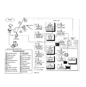
Figure 1 illustrates a representative system embodiment of the present
invention.
Figure 2 shows an overall schematic of the Energy Hub Management System (EHMS)
of the
present invention, in one embodiment thereof.
Figure 3 shows an example of a residential micro hub structure layer of the
EHMS.
Figure 4 shows a further implementation of the EHMS in a residential context.
Figure 5 shows an illustrative comparison of forecasted and actual power
generation from gas
fired plants on a winter weekday.
Figure 6 shows an illustrative comparison of forecasted and actual power
generation from coal
fired plants on a summer weekday.
Figure 7 shows an illustrative comparison of forecasted and actual power
generation from gas
fired plants on a summer weekday.
3
CA 02831621 2013-09-27
WO 2012/129675 PCT/CA2012/000319
Figure 8 shows an illustrative comparison of indoor temperatures of Case 0 and
Case 1.
Figure 9 shows an illustrative operational schedule of the air conditioner in
Case 1.
Figure 10 shows an illustrative comparison of inside fridge temperature in
Case 1 and Case 0.
Figure 11 shows an illustrative operational schedule of fridge.
Figure 12 shows an illustrative comparison of water temperature in Case 1 and
Case 0.
Figure 13 shows an illustrative operational schedule of water heater.
Figure 14 shows an illustrative comparison of power consumption of lighting in
Case 1 and
Case 0.
Figure 15 shows an illustrative comparison of operational schedule of
dishwasher in Case 1 and
Case 0.
In the drawings, embodiments of the invention are illustrated by way of
example. It is to be
expressly understood that the description and drawings are only for the
purpose of illustration
and as an aid to understanding, and are not intended as a definition of the
limits of the
invention.
DETAILED DESCRIPTION
The present invention provides a system and method for energy management. The
energy
management system of the present invention is provided by a platform that
enables an energy
hub and system for dynamic management of the energy hub. The energy hub
interfaces with
various energy components at a particular premise, such as various energy
consuming devices.
The system of the present invention includes an energy optimization engine
that is operable to
generate an energy model that optimizes energy usage of energy consuming
components
based on energy component models, external and environmental data, previously
generated
energy models and user preferences.
The present invention solves the problem of conservation and demand management
(CDM) by
modeling energy loads of industrial, commercial and residential users,
including by modeling
energy components and energy demand, cost and carriers. Thus it is possible to
minimize
energy consumption, environmental footprint and/or cost, and maximize profits
in the case of
demand response programs. For example, an industrial consumer that owns a
micro-turbine
may at certain times during their daily operation decide not to turn the
turbine on, as the energy
4
CA 02831621 2013-09-27
WO 2012/129675 PCT/CA2012/000319
cost differential between electricity and gas might not justify it, even if
demand response
programs are taken into account. However, if the use of the heat generated by
the turbine can
supply part of the thermal demand, the present invention may determine that it
is optimal to turn
on the turbine.
Figure 1 illustrates a system in accordance with the present invention. An
energy hub is linked
to an energy optimization engine that is operable to generate an energy model.
The energy hub is further linked to one or more energy components at a
particular premise,
such as a residence, commercial centre or industrial centre. Energy components
models may
be provided by a device database linked to the energy hub. Energy component
models may be
provided by measuring past behaviour of the energy component (heuristics)
and/or by predicted
information supplied by a manufacturer or reseller.
The energy hub provides bidirectional control of the energy components,
including recording
energy utilization (consumption/production/storage) data and directing
operation of the energy
components. Energy components may be energy consuming devices, energy storage
devices
and/or energy producing devices.
The energy hub may also be linked to an external and environmental data
source, which may
be located remotely from the premise and accessed by the energy hub by network
connection,
such as over the Internet. External and environmental data may include local
electricity
conditions, electricity market prices and weather forecasts.
The energy hub further includes or is linked to a user interface that enables
an energy manager
(a user) to indicate user preferences that are used to generate the energy
model. The user
interface may be a web-based user interface accessible by a computer linked by
network to the
energy hub.
The energy hub may further be linked to one or more smart meters for obtaining
energy usage
information for the premise or for other locations.
The energy hub is not limited in size and can range from a single household
energy system up
to an entire city energy system, considered as a single hub. The energy hub of
the present
invention may be applied in a number of energy utilization sectors including:
residential (e.g.,
single detached houses), commercial and institutional (e.g., retail stores,
shopping malls,
schools, hospitals), industrial (e.g., paper mills), agricultural (e.g., dairy
farms).
CA 02831621 2013-09-27
WO 2012/129675 PCT/CA2012/000319
In any electric energy system, the customers' objective is to minimize their
energy cost, whereas
utilities are not only concerned about the cost, but also issues such as load
shape, peak load,
quality of service, etc.
In accordance with the energy hub of the present invention, as shown in Figure
1, a two-tier
system architecture is provided that in part enables the differentiation of
the objectives of
customers and the utility. At the lower level, or i.e., micro hub level, the
objective is to optimize
the energy utilization from the customer's point of view, whereas at the macro
hub level, i.e., a
group of micro hubs controlled and scheduled together (e.g., a group of
detached house micro
hubs), the objective is to optimize the energy utilization from the utility
point of view.
At the macro hub level, operational decisions are taken for a group of micro
hubs which are
passed on to each micro hub for the next scheduling horizon. The micro hub
implements the
received schedule in real-time and monitors the energy utilization and
operational status. If for
any reason the schedule is not followed, the micro hub may generate a new
schedule for the
rest of the scheduling horizon.
It should be understood that the macro hub layer is operable to provide co-
ordination and
control. In some implementations, the macro hub layer may have the authority
to enforce
specific rules (for example related to energy utilization) in connection with
the micro hubs. For
example, electric vehicles are gaining in popularity but transformers and
other components of
the energy grid are designed in a way that if a sufficient number of people
sought to charge
electric vehicles at the same time the stress on the grid could result in for
example transformer
burn-out.
It should be understood that micro hubs may be assigned to macro hubs based on
power levels,
average consumption and other factors. Generally speaking, the macro hub may
be
implemented on a one per substation or one per feeder basis. Limits may be set
to the number
of micro hubs associated with each macro hub.
The EHMS is operable to remove some of autonomy of the micro hubs, not just by
virtue of the
central controller, but by operation of control that is distributed by
operation of the present
invention between the central controller and for certain local operational
matters, the applicable
macro hub. For example an optimizer may be implemented to the system, which
may be
implemented to the macro hub layer and optionally also to the central
controller, such that the
optimizer function is distributed as between the macro hub layer and the
central controller.
6
CA 02831621 2013-09-27
WO 2012/129675 PCT/CA2012/000319
In one particular implementation, the optimizer is implemented to the macro
hub layer, based on
configurations determined for the operator of the overall grid, but the
control operations
associated with the functioning of the optimizer may be trumped by for example
network
broadcast messages from the central controller, for example peak demand
constraint related
broadcast messages. The optimizer is also implemented to the micro hub layer,
and in one
aspect a hierarchy may be established in the configuration of the system such
that the macro
hub layer is operable to override operation of the micro hub layer. In one
aspect of the system,
it is not necessary that the optimizer in the micro hub layer and the
optimizer of the macro hub
layer be linked, rather it is the micro hub layer that operationally linked to
the macro hub layer as
described herein.
The localization, or localization in part, of control of energy delivery and
consumption, by virtue
of the EHMS architecture, incorporating the macro hub layer as described
below, provides an
effective way to provide smart grid advantages including better utilization of
energy resources.
The macro hub layer described may be operable to enforce particular
optimization rules and
thereby provide improved energy management solutions for localized problems
that affect or
may affect the feeder level of the energy grid. The system described also
enables on demand
solutions such as payment for premium access to energy resources based for
example on tier
pricing regime.
Optimization may be implemented by operation of the micro hub controller, but
the micro hub
controller may dynamically obtain instructions that enable control from a
cloud network. It
should be understood that whereas optimization could be run on the micro hub
controller but it
could also be run in the cloud ¨ the controller could dynamically obtain the
instructions from a
remote computer or remote network such as a cloud computing network linked to
the EHMS.
Therefore, it should be understood that while the architecture described
contemplates the macro
hub and micro hub layers, each being operable to enable control functionality,
each of these
layers may also be linked to further resources in exercising their respective
control operations,
for example a cloud computer network.
Figure 1 shows the overall architecture that provides the macro hub and
plurality of associated
microhubs. The architecture enables the interaction between these hubs by
means of the
overall Energy Hub Management System (EHMS) described herein, including the
data and
information exchanges that are facilitated between the hubs.
The EHMS described herein a solution that allows static energy users to
effectively manage
their energy requirements. More specifically, the EHMS empowers energy hubs ¨
that is,
7
CA 02831621 2013-09-27
WO 2012/129675 PCT/CA2012/000319
individual locations that require energy (e.g., manufacturing facilities,
farms, retail stores, but
specifically in this case detached homes) in a way that they can contribute to
the development
of a sustainable society through the optimal real-time management of their
energy demand,
production, storage and resulting import or export of energy.
The EHMS may be implemented using the following elements:
= Two-way controls on energy consuming and producing devices within the
energy hub. In
on aspect, these controls may have the capacity both to record, as
appropriate, energy
utilization (consumption/production/storage) data and to direct the operation
of the
individual device.
= A central core or controller through which the information collected from
the energy
hub's devices, the external environment (for example, local electricity
conditions,
electricity market prices and weather forecasts) and the models developed from
past
device performance are used in user-defined decision-making heuristics in
order to
manage energy effectively.
= Optionally a web-based portal is provided acts as an interface between
the energy hub's
managers and the central core/device technology. The present invention may be
implemented using state-of-the-art wireless communication devices, cloud
deployment
and various instrumentation and control technologies, and thereby provides an
effective,
integrative interface amongst energy producing and consuming devices within a
single,
static location. The web-based portal may be configured and presented in a
user-
friendly portal for managers of the energy hub for local use or remote use.
Referring to Figure 1, the following described in greater detail the principle
elements of the
architecture shown in Figure 1, which is one possible implementation of the
present invention.
Micro-hub Controller (pHC)
This element is best understood as an embedded computing device (using
hardware and
software suitable for the applications described, configured in a manner
obvious to those skilled
in the art), installed within a home (or other particular location),
configured to enable one or
more of the following (and other operations are possible):
= Communicating with the utility smart meter(s), typically via a wireless
communications
protocol such as an IEEE 802.15.4 variant, to acquire real-time energy
utilization, price
information schedules, etc.
8
CA 02831621 2013-09-27
WO 2012/129675 PCT/CA2012/000319
= Acquiring energy utilization data from various "smart" endpoints (e.g.
load control
devices, smart thermostats, smart appliances, smart breaker panels, local
energy
sources), typically, but not necessarily, through a wireless communications
protocol (e.g.
Zigbee HA/SE).
= Communicating with Data Centre (see below) bound applications to receive
various
optimization inputs (e.g. predicted energy price trajectories, kWh related
carbon
predictions, weather forecasts, historic anal data of a similar nature, device
model
parameters, and optimization objectives).
= Computing an optimal energy hub device optimization schedule subject to
energy hub
manager defined preferences and optimization objectives, as per the
methodology
defined herein (this computation may optionally occur on servers at the Data
Centre and
be delivered securely to the pHC over the public internet)
= Automatically and reliably sending requisite control signals to the
elements under direct
control according to the computed optimal operations schedule, and presenting
said
schedule to the Energy Hub Manager for discretionary control items i.e.
devices for
which the energy hub manager has elected not to provide a control endpoint, in
multiple
forms (e.g. in home display, portable digital assistant (PDA) / smart phone,
web portal.
This may also include the enablennent of alternative generating sources within
the
energy hub, and/or storage assets.
= Locally storing and then forwarding to the Data Centre normalized energy
utilization and
load profile data for all metered elements within the energy hub.
= Receiving co-ordination and control instructions (e.g. additional
optimization constraints,
operating refinements) from its associated macro-hub controller, should there
be one,
and forwarding information like projected load profile such that macro-hub
level
optimizations can also be carried out (e.g. adjusted electric vehicle charger
operating
schedule).
Macro-hub Controller (@HC)
A computing device, possibly installed within a residential neighbourhood (or
other local energy
service area) in close proximity to its electricity distribution system,
(using hardware and
software suitable for the applications described, configured in a manner
obvious to those skilled
in the art), configured to enable one or more of the following (and other
operations are possible):
9
CA 02831621 2013-09-27
WO 2012/129675 PCT/CA2012/000319
= Sensing localized grid / distribution system status data e.g. current
transformer loading
levels, tap changer positions.
= Sending control signals to the local distribution system to effect
optimal equipment
operation.
= Secure, bi-directional communications with a set of associated pHC's to
ensure their
individual micro-hub level optimizations factor local grid conditions.
Data Centre
The system may be linked to a data centre (provided in a manner known to those
skilled in the
art) for remote logging of relevant information including for example energy
utilization data and
device status data. The data centre may enable the functionality described
below, and include
the components described below.
= Micro-hub / Macro-hub (pHC / @HC) Connectors: modules capable of secure
communications with remotely installed and micro and macro hub controllers,
primarily
for the purpose of energy utilization data and device status information.
= Data Quality Assurance: a software module that ensures the quality of the
data sourced
from the pHC's e.g. detecting anomalous / erroneous energy data values with
optional
capability of providing reasonable substitute according to a number of
possible
substitution algorithms.
= Energy Price Predictor a module capable of providing reliable hourly
predictions of near-
term energy spot prices (e.g. for the coming 24 hours).
= Carbon factor Predictor: a module capable of generating hourly
predictions of near-term
hourly carbon factors per kWh based on the predicted generation mix within the
jurisdiction.
= Modelling Engine / Parameter Export: optimizer related software module
capable of
serving requests (e.g. via a web service API) from authenticated pHC's to
provide user
defined and system defined optimization model parameters, constraints and
objectives,
and possibly computing the optimal operations schedule.
= Web Portal / Data Visualization: a set of software modules that provides
Energy Hub
Managers a secure viewport into their system, possibly from a home computer,
their
CA 02831621 2013-09-27
WO 2012/129675 PCT/CA2012/000319
smart phone, etc. to monitor system status, adjust preferences and
optimization
objectives, set and track "energy budgets / goals", enable over-rides, etc.
= External Data Collector a module capable of interfacing with all required
external data
sources (e.g. the system operator, a weather forecasting service) and storing
this
information in a central repository available for use by other Data Centre
applications.
= Notification Engine: a service capable of providing relevant
notifications to Energy Hub
Managers (e.g. system status changes, availability of new optimal operations
schedules)
through a variety of configurable notification devices (e.g. e-mail, social
networking
sites).
= Scheduler: a module that facilitates scheduling services for activities
like periodic pHC
/@HC interactions, optimizer runs, etc.
Figure 2 also shows the three other categories of the macro hubs, namely,
commercial and
institutional, agricultural, and industrial. In these macro hubs, there may or
may not exist
multiple micro hubs, but all would have similar arrangements for data and
information exchange.
As seen in Figure 3, a typical residential macro hub will comprise several
micro hubs which
would communicate with the macro hub with regard to their energy usage and
control decisions.
The micro hubs are at the residential household level and the macro hub can be
thought of as a
group of residential micro hubs. Figure 4 also shows a representative
residential
implementation, also illustrating integration of the system of the present
invention with third
party devices.
In one aspect of the invention, each micro hub is operable to generate its
operational schedule
as per one or more models, for example the ones discussed herein. The
generated schedules
may be communicated to a macro hub linked to the micro hub, and which
incorporates this
information and system level information to execute a macro-hub level
operational model. The
outcomes from the macro-hub level will be sent back to the micro hubs which
then apply these
as outer bounds on constraints of their micro-hub operational model.
The present invention therefore provides a multi-level optimization technology
that involves
coordination between the sectoral macro hub and the multiple micro hubs within
each macro
hub. The system infrastructure that includes at least one macro hub and
multiple associated
micro hubs is operable to embody or implement one or more models for optimal
operation of
macro hubs for example for the four categories described, and which
incorporate a series of
optimization operations from both the customer and the utility point of view.
The models
11
CA 02831621 2013-09-27
WO 2012/129675 PCT/CA2012/000319
incorporate a series of rules or processes for determining whether customer
driven or utility
driven factors shall govern in particular circumstances, within a particular
time period.
The macro hub controller is operable to establish a view of local conditions
across a plurality of
associated micro hub controllers. These conditions include for example local
demand and cost
saving objectives of local home owners. These conditions are captured and
analyzed on a real
time or near real time basis. The macro hub is in communication with the
operator, and is
operable to obtain information regarding pricing and demand objectives of the
operator. The
macro hub includes functionality that enables the balancing of these consumer
and operator
objectives based on current local conditions and also current objectives of
the operator.
The energy optimization engine generates an energy model based on one or more
energy
component models, external and environmental data, previously generated energy
models
and/or user preferences. The energy optimization engine may implement a mixed
integer linear
programming (MILP) optimization model for optimal operation scheduling of the
energy hub.
The optimization model can be configured to minimize demand, total cost of
electricity, gas or
other utilities, emissions and peak load over the scheduling horizon while
considering the user
preferences. Thus, the MILP optimization model can be configured to optimize
energy usage
based on electricity usage, gas usage, human comfort factors, greenhouse gas
emissions,
price, etc.
The scheduling horizon used by the energy optimization engine can vary, for
example from a
few hours to days, and the selection depends on the type of the energy hub and
types of
activities which take place in the energy hub. For example, in a residential
energy hub the
scheduling horizon could be set to 24 hours with 1 hour to a few minutes time
intervals. Without
any loss of generality, in the present specification a 24 hour scheduling
horizon with time
intervals of 15 minutes have been used, with the exception of the fridge which
is 7.5 minutes
due to its thermodynamic characteristics.
The optimization model may be solved using any MILP solver such as GNU Linear
Programming Kit (GLPK) freeware solver or commercial solver CPLEX.
An example of an optimization model is provided herein for a typical
residential application,
including major household demands and energy storage/production system is
developed. The
developed model incorporates electricity and gas energy carriers, and takes
into account human
comfort factors and green house emissions. The objective functions of the
model and
12
CA 02831621 2013-09-27
WO 2012/129675 PCT/CA2012/000319
operational constraints associated with the energy components of the energy
hub are explained
in detail here.
A general form of the optimization model for the residential sector may be as
follows:
rnin J = Objective function
(2.1a)
S ) < P(t)
ma
s.t. (t
et , T (2.1b)
iGA
Device i operational constraints
Vi e A (2.1c)
Constraint (2.1b) sets a cap on peak demand of the energy hub at each time
interval, and
ensures that maximum power consumption at a given time does not exceed a
specified value.
The peak-power limit in this constraint could be set in such a way that the
utility can take the
advantage of peak-load reduction from each energy hub during peak-load hours.
During off-
peak and mid-peak hours of the power system this constraint may be relaxed.
Depending on the user preferences, different objective functions can be
adopted to solve the
optimization problem. Thus, minimization of the customer's total energy costs,
total energy
utilization, peak load, emissions and/or any combinations of these over the
scheduling horizon
may be considered as possible objective functions for the optimization model.
The following objective function for the residential energy hub corresponds to
the minimization
of the user's total energy costs over the scheduling horizon:
=j2 CD(t) Si(t) E CD(t) Puz Suz(t) Lz (t)
teT iGA zGLI
ic1{LI,ESD.PV}
_ E Gs(t)PS(t)+ E CG(t) S(t) (2.2)
iGIESD.P1/1 ic{11,1V11}
The first two terms in (2.2) represent the cost of electricity consumption,
the third term
represents the revenue from selling stored/produced electricity to the power
grid, and the last
term represents the cost of gas consumption.
An objective function for minimization of total energy consumption over the
scheduling horizon
may be represented as follows:
13
CA 02831621 2013-09-27
WO 2012/129675 PCT/CA2012/000319
-12 = E p Si(t) + > PLiz sm, I L,(t)
teT icA 2e1,/
i4{LI,ESD,P17}
- E Pi Si (t) + > HR (t) (2.3)
ic{Esapv} ie{11,1171/}
This minimizes operational hours of all devices and maximizes the operation of
energy
production/storage devices. In this case, the energy price has no effect on
the optimum
schedule.
An objective function for minimization of green house emissions may be
formulated using the
social cost of CO2 at each hour as follows:
E C Ern (t) Pi Si (t) + E cEm(opL, sm, (t) II(t)
ter iept zeLl
iV{LI,ESD,PV}
- E cEm(t) Pi Si (t)
(2.4)
Here, it is assumed that the electricity injected to the grid by the ESD is
emissions free.
An objective function for minimization of peak load can be adopted to reduce
the demand of the
energy hub as follows:
=
si(o+ E pm, suz (t) I L õ(t) Vt G T
(2.5)
iGA zeLl
In addition to the aforementioned individual objective functions, any
combinations of these
objective functions can also be used as the objective function of the
optimization model. Thus,
appropriately weighted linear sum of the objective functions J1, J2, J3, and
J4, can be used as an
objective function of the optimization model as follows:
14
CA 02831621 2013-09-27
WO 2012/129675 PCT/CA2012/000319
J = k2J2 + k3J3+
(2.6)
where kl represents the weight attached to the customer's total energy costs
in the objective
function; k2 converts the total energy consumption in kWh to cost in $ and
specifies its weight; k3
represents the weight of the total emissions costs, and k4 represents the
effect of the peak load
in $ and its weight in the objective function.
To provide an accurate energy model, each energy component linked to the
energy hub is
represented by an energy component model. For a typical residential energy
hub, three
categories of components can be identified: energy consumption, energy
storage, and energy
production. Each of these components has its own specific behaviour,
operational constraints,
and settings required to operate appropriately. Recognizing the components'
behaviour is very
important in order to identify and define the decision variables, and
formulate the optimized
model constraints. In other words, the energy optimization engine must know
what kind of loads
(devices) are connected in the energy hub in order to take actions according
to the behaviour of
the load.
The energy components models optimally give priority to user preferences, and
are simple
enough for successful implementation and easy interpretation of the results.
For example,
energy component models in the residential sector may include the following
parameters in
order to capture most of the aspects of the customer preferences:
= the normal temperature or ambient energy (ambient criteria);
= the maximum temperature deviation that the customer is willing to
tolerate
(comfort criteria);
= the distribution of the cycle able load; and
= residential thermal loss.
Energy component models should fulfill at least two objectives when evaluating
Demand Side
Management (DSM) policies: first, they should provide the necessary
information to evaluate
the benefits of DSM implementation, and second, they should provide some
comfort index in
order to evaluate every control action from the end-user. Considering the
above mentioned
aspects, energy component models for major energy components in a residential
setting are
provided herein.
CA 02831621 2013-09-27
WO 2012/129675 PCT/CA2012/000319
Furthermore, various dynamic pricing methods may be available to electricity
customers in the
residential sector, including Fixed Rate Plan (FRP), Time-of-Use (TOU)
pricing, and Real-Time
Pricing (RTP).
In FRP there is a threshold that defines higher and lower electricity prices
for customers. If the
total electrical energy consumption per month is less than the threshold, then
the customers pay
the lower price as a flat rate; if it exceeds the threshold, they pay the
higher price for each
kilowatt hour. For example, in Ontario the threshold is currently set at 600
kWh per month in the
summer and 1000 kWh per month in the winter for residential customers and 750
kWh per
month for non-residential customers. The difference in the threshold values
recognizes that in
the winter, Ontario's customers use more energy for lighting and indoor
activities and that some
houses use electricity heating.
TOU pricing is the simplest form of dynamic pricing. The main objective of
dynamic pricing
programs is to encourage the reduction of energy consumption during peak-load
hours. In TOU
pricing, the electricity price per kWh varies for different times of the day.
In Ontario, TOU pricing
is currently based on three periods of use of energy:
= on-peak, when demand for electricity is the highest;
= mid-peak, when demand for electricity is moderate; and
= off-peak, when demand for electricity is the lowest.
The classification of On-peak, Mid-peak, amid Off-peak periods vary by season
and day of the
week.
In RTP, the price varies continuously, directly reflecting the wholesale
electricity market price
and are posted hourly and/or day-ahead for pro-planning. It provides a direct
link between the
wholesale and retail energy markets and reflects the changing supply/demand
balance of the
system, to try to introduce customers price elasticity in the market.
In the residential sector, the occupancy of the house may also have a major
effect on energy
utilization patterns. Furthermore, energy utilization patterns differ in each
house depending on
the season, and the day such as weekdays and weekends. To consider the effect
of household
occupancy on energy utilization patterns, a new index termed as the Activity
Level may be
defined for electrical appliances. This represents the hourly activity level
of a house over the
scheduling horizon.
16
CA 02831621 2013-09-27
WO 2012/129675 PCT/CA2012/000319
To determine a reasonable value of the Activity Level of a residential sector
energy hub,
historical data of energy utilization provided by installed smart meters at
each house can be
used. Smart meters can provide a wealth of data, including energy consumed
each hour or
even in each fifteen minute interval. Therefore, the measured data of the
previous weeks,
months, and years can be used to predict the energy utilization on a
particular day.
Statistical methods can be used to construct household load profiles on an
hourly basis.
Similarly, load models may be developed using a linear regression and load
patterns approach.
The load pattern may be represented as the sum of daily-weekly components,
outdoor
temperature, and random variations. These load patterns could be modified to
obtain the
proposed Activity Level of a house on an hourly basis.
It should be noted that the Activity Level index has a different effect on
each of the electrical
appliances in the house. For example, the effect of the activity level on the
fridge temperature is
not the same as its effect on the room temperature. Thus, the Activity Level
index is related to
each of the energy consuming devices with an appropriate coefficient.
During base-load hours of the house, which represents time periods of
inactivity inside the
house, occupants are either sleeping or outside the house, and therefore the
probability of the
fridge door being opened is zero. By inspection, the value of this base-load
consumption is
approximately 50% of the average hourly electrical energy consumption.
Therefore, to
determine the fridge activity level, ALFR, it can be assumed that the base-
load consumption is
50% of the average household consumption; thus, any load that is less than the
base-load will
not contribute to the fridge activity.
Another environmental data item is green house gas emissions. Electric systems
in general
depend on various generating units which include nuclear, hydro-electric, gas
and coal power
plants, and some amount of renewable energy resources. Typically, nuclear and
large hydro-
electric units provide base load generation. Coal and gas-fired generating
units, which are
responsible for CO2 emissions, generally run during the day and supply a part
of the base load,
but mostly supply peak load. Coal and gas produce different amounts of CO2
therefore, power
generation from coal and gas-fired generating units needs to be known in order
to estimate the
CO2 emissions from the system.
A power generation forecast may be one of the external data items. The system
operators, e.g.,
the Independent Electricity System Operator (IES0), do not typically provide
power generation
forecasts for power plants. Therefore, the power generation from coal and gas-
fired generating
17
CA 02831621 2013-09-27
WO 2012/129675 PCT/CA2012/000319
units may need to be forecasted. Rather than considering each individual unit
separately, the
estimation can be done by considering the aggregate generation from coal-fired
plants and from
gas-fired plants, separately. These forecasts may be carried out using an
econometric time-
series model.
External inputs required by the forecasting model may be as follows:
= a 24-hour ahead total system demand profile obtained from pre-dispatch
data;
= hourly total system demand for the past 14 days; and
= hourly cumulative generation from coal- and gas-fired units for the past
14 days.
The following time-series forecasting model is used to forecast the power
generation from coal-
and gas-fired power plants in Ontario for example, separately:
fit,p = Yit,p nt (kt Xt) Vt c {1,2, = = . 24},Vp {coal, gas} (1.1a)
1 Ti
Vt G {1,2,, = = ,24},Vj {1,2, = = = ,14} (1.1b)
Ytp
1 n
= ¨ E Vt {1,2,¨ = ,2-1},Vj E {1,2, = = = .1,1},Vp G
{coal, gas}
(1.1e)
En_1173 t (X i t ¨ &wan)
Bt = " Vt c {1,2, = = = ,24},Vj G {1,2, = = = ,1.1},Vp c
{coal gas}
Ejn=1 (-K21 man)
(1.1d)
An emissions forecast is another external or environmental data item. Natural
gas and coal
have different chemical compositions and hence produce different amount of
CO2. Natural gas
is the least carbon-intensive fossil fuel, and its combustion emits 45% less
CO2 than coal.
Therefore, separate rates of emissions for gas and coal fired units have been
used. The day-
ahead emissions profile is calculated as follows:
Em(t) = R, x Pe(t)+ fig X Pg(t) Vt e {1, 2, = = , 241
(1.2)
18
CA 02831621 2013-09-27
WO 2012/129675 PCT/CA2012/000319
The marginal cost of CO2 emissions per kWh energy generation may be
calculated, for
optimization purposes, using the Social Cost of Carbon dioxide (SCC) emissions
or marginal
damage cost of climate change, as follows:
Ern(t) x )SCC
CE,,,i(t) = __________________________ Vt G 11, 2, = = , 24}
(1.3)
jc(t
Using the forecasted data, a day-ahead emission profile can be calculated.
Examples
Energy component models of major household devices (appliances), i.e., air-
conditioning,
heating system, water heater, pool pumps, fridge, dishwasher, washer and
dryer, and stove are
provided herein. Also, a generic energy component model for energy
storage/generation
devices, and an energy component model of a photo-voltaic (PV) solar array is
provided. These
set of energy component models represent the operational constraints of the
residential energy
hub. The definition of the model variables and sample parameter values are:
19
CA 02831621 2013-09-27
WO 2012/129675 PCT/CA2012/000319
Indices Description Example
Device (Appliance) i = FR, i = AC
Time interval t = 1, 2, 3, , 96
Sets Description Example
A Set of devices (appliances) {ER, AC, H, DIV, WI
Set of indices in the scheduling horizon T {1. .. 96}
C T is the set of periods in which device i may op- TAr = {1 . 96}
erate; T = It E T : E0T2 <t < LOTzl
Variables Description Example
S(t) State of device i at time t, binary On/Off
(t) Binary- variable denoting start. up of device i at tune 1: 0/1
1 startup of device i at time t
tli(t) =
0 Otherwise
Binary variable denoting shut down of device i at time 0/1
1 shutdown of device i at time t
0 Otherwise
Or (f) Temperature of device i a time t Op(t)
IL(t) Illumination Level of a given zone z in the house at time
L(z,t) e {1, = = = ,6}
ESL(t) Energy Storage Level of device i at t ESLESD(t)
Parameters Description Example
CD/0 Price of electricity demand at time t TOU electricity price
Cs(t) Price of electricity supply at time t Fixed electricity price
(80 cents/kWh)
Ca(t) Price of gas demand at time t Fixed gas rate (25 cents/m3)
CEm(t) Marginal cost of emissions at time t 7 cents/kWh
Maximum allowed peak load of the energy hub at time 10 kW
Rated power of device i PPR = 350W
EOTi Earliest Operation Time of device i EOTFR = 1
LOT Latest Operation Time of device i LOTFR = 96
MUT, Minimum Up Time of device i AfUTFR = 2 (2 time
intervals)
MDT Minimum Down Time of device i AI UTF R = 2 (2 time
intervals)
A/ SOTt Maximum Successive Operation Time of device i AISOTstv = 3
AL(t) Activity Level at time t Figure 1.3
ALER(t) Activity Level of fridge at time t Figure 1.4
H L (t) Average hourly Hot Water Usage at time t Figure 2.1
HI? i Heat Rate of of device i HRwn = 3m3 per time interval
0,4P Upper limit of temperature of device i Oup = 4 C
f`
0 Lower limit of temperature of device i O' ' = 1.5 C
R
I Lzm(t) Minimum required zonal illumination at time t Figure 2.3
Outdoor illumination level of a given zone in the house Figure 2.4
at time t
E nrin Minimum Energy Storage Level of device i ESI min = 250 Wh
'PSD
ES LT' Maximum Energy Storage Level of device i ES L"EH" = 3000 Wh
SD
C H Charged energy into device i at time interval t CHpv(E)
DC H Discharged energy from device i during one time interval DC H
F,'SD = 100 Wh
LPN Large Positive Nurnber LPN = 1000
Fridge
In order to model the operational aspects of a fridge for scheduling purposes,
both the variable
under control and operational constraints of the fridge should be considered.
The developed
model should be able to maintain the fridge temperature within a specified
range, while taking
into account technical aspects of the fridge operation as well as the customer
preferences. The
operational constraints of the fridge in the optimization model are as
follows:
CA 02831621 2013-09-27
WO 2012/129675 PCT/CA2012/000319
{ 0
S(t) = or 1 if t c = FR
i(
(2.7a)
0 if t = FR
{
= = 1 if O (2.713
FR(t = 0) > OFt'PR
Si(t 1) )
0 if OFR(t = <
01A OFR(t) 5- OFul
Vt cT. i = FR (2.7c)
OFR(t) = OFR(t ¨ 1) + /3FR A1(t) ¨ aFR
'YFR Vt T,i = FR (2.7d)
The time period over which the fridge can be in operation is specified by
(2.7a), where the
customer defines the EOT amid the LOP of the fridge. Equation (2.7b) ensures
that if the fridge
temperature at t = 0 is more than the upper limit, as specified by the
customer, the fridge state is
On in the first time interval. Constraint (2.7c) ensures that the fridge
temperature is within the
customer's preferred range.
Equation (2.7d) relates the temperature of fridge at time t to the temperature
of fridge at time t ¨
1, activity level of the fridge at time t, and On/Off state of the fridge at
time t. The effect of the
activity level on fridge temperature is modeled using OFR so that as the
household activity level
increases, the temperature increases. In other words, more activity in the
house results in more
cooling demands for the fridge.
The effect of the On state of the fridge on fridge temperature reduction is
represented by aFR,
and the warming effect of the Off state of the fridge is modeled by yFR. The
latter is to address
the thermal leakage because of difference in temperatures of the fridge and
the kitchen. The
parameters PFR, aFR, and yFR can be measured or estimated from simple
performance tests. The
same model with different coefficients and parameter settings can be used to
model the freezer
in a household.
Air Conditioning (AC) and Heating
Operational constraints developed for modeling of the heating system in a
house are similar to
the operational constraints of the AC. Therefore, the AC and heating system
constraints are
presented using a common set of equations, as follows:
21
CA 02831621 2013-09-27
WO 2012/129675
PCT/CA2012/000319
{ Or 1 if t G Ti, = AC I H
S (t) =
(2.8a)
0 if t Ti, = AC /
Si(t = 1) = 1 if Oiõ(t = 0) > 07õ = AC
(2.8b)
0 if 8(t = 0) < , = AC
((t = ) = I if Oin(t = 0) < = H
S 1 2.8c
i )
0 if O(t = 0) > i H
< Oin(t) < 0 junP
Vt c T, i = AC /H (2.8d)
O(t) = Oin(t ¨ I) + f3Ac AL(t) ¨ aAcSi(t)
7Ac(000(t) ¨ (t)) Vt c T, i = AC (2.8e)
(t) = Oin(t ¨ 1) + ,13H AL(t) + oHSi(t)
H in(t) 0 Out(t)) Vt c T,i=
H (2.8f)
In the proposed operational model, the time period over which the AC (or the
heating system)
can be in operation is specified by (2.8a), which is specified by the
customer's E07; and LOP;
settings. Equation (2.8b) ensures that if the indoor temperature at t = 0 is
more than the upper
limit, as specified by the customer, the AC state is On in the first time
interval, and (2.8c)
ensures that if the indoor temperature at t = 0 is less than customer defined
lower limit, the
heating system state is On in the first time interval. Constraint (2.8d) is
included in the model to
maintain the indoor temperature within the customer preferred range.
Equations (2.8e) and (2.8f) represent the dynamics of indoor temperature for
time AC and the
heating system, respectively In these equations, 00,(t) is the forecasted
outdoor temperature at
time interval t of the scheduling horizon. These equations state that the
indoor temperature at
time t is a function of the indoor temperature at time t ¨ 1, household
activity level at time t,
On/Off state of the AC (H) at time t, and the outdoor and indoor temperature
difference. The
effect of the activity level on indoor temperature increase is modeled by PAc
(3H). Also, PAC (PH)
represents the effect of outdoor and indoor temperature difference on indoor
temperature.
The cooling and warming effect of an On/Off state of the AC (the heating
system) on indoor
temperature are represented by aAc and VAC (aH and yH), respectively. The
developed model
captures the normal temperature (ambient criterion), and time maximum
temperature deviation
that time customer is willing to tolerate (comfort criterion).
22
CA 02831621 2013-09-27
WO 2012/129675 PCT/CA2012/000319
Water Heater
An average hourly hot water usage pattern, which is available in the prior
art, can be considered
for each individual house. There is a larger and earlier spike on weekdays'
consumption
patterns, whereas the spike occurs later and is significantly flatter on
weekends.
The operational constraints of the water heater are represented by:
{ 0 or 1 if t = 117/
Si (t) =
(2.9a)
0 if t =
,Si(t = 1) = 1 if Own(t = 0) <
(2.9b)
0 if Otvii(t = 0) > (CH
011 I,111/' < 011,H (t) Vt c Ti = 1.1711
(2.9c)
011'11(0 = OviTH (t ¨ 1) ¨ ,3117] HWU(t)
+ awl/S(t) ¨ 711-1/ Vt e T,i = TVH
(2.9d)
The basic operational constraints of the water heater are similar to those of
the fridge and AC
model, and are given by (2.9a)- (2.9c). Constraint (2.9d) assumes that the
dynamic relation of
the water heater temperature at a given time interval t is a function of the
water temperature at
the previous time interval, the average hot water usage, and the On/Off state
of the water heater
at time interval t.
Hot Tub Water Heater
The operational constraints of the water heater can also be used for a hot tub
water heater. The
only difference between these models is in their parameter settings such as
average hot water
usage, temperature settings, operational time, and associated coefficients
that may have
different values.
0 or 1 if t E = T14711
0 if t Ti, i = TIM
(2.10a)
Si(t = 1) = 1 if 07-wIt(t = 0) < OMTH
(2.101))
0 if !hurl/ (t = 0) > H
8TI < TWO) < OTuP14' Vt E Ti, i = T1V H
(2.10c)
Orwx (t) = 0 714,- H (t ¨ 1) ¨ 07- w H HIV U (t)
+ anvil Si (t) ¨ 2TWH V t c Ti = TWI/
(2.10d)
23
CA 02831621 2013-09-27
WO 2012/129675 PCT/CA2012/000319
Dishwasher
The proposed operational model for the dishwasher is as follows:
0 or 1 if t c= DIV
Si(t) =
(2.11a)
0 if t T. i = DIV
U(t) ¨ Di(t) = S i(t) ¨ Si(t ¨ 1) et c T, i = DIV
(2.11b)
U(t) Di(t) < 1 et c Ti = DIV
(2.11c)
E (k) = ROTi et c Ti = 1V
(2.11d)
teTi
t+111LITi
Si(k) > MUT ¨ LP N (1 ¨ Lri(t)) et G Ti = DIV (2.11e)
k=t
M SOTi
Si(k) < M SOTi + LPN (1 ¨ U(t)) et c Ti = DIV
(2.11f)
k=t
In this model, the time period over which the dishwasher can be in operation,
which is specified
by the customer's EOT and LOP settings, is specified by (2.11a). The required
operation time,
minimum up time, and maximum successive operation time of the dishwasher are
parameter
settings specified by the end-user, and are modeled by (2.11d) to (2.11f),
respectively.
Washer and Dryer
The proposed operational models for washer and dryer are similar to the
proposed model of
dishwasher. The set of constraints for the washer and dryer is as follows:
{ 0 or 1 if t G = {W, DRY}
Si(t) = 2.12a
0 if t Ti, i = D RY } ( )
Ui(t) ¨ Di(t) = Si(t) ¨ Si(t ¨ 1)
et E Ti, = {W, DRY} (2.12h)
U(t) Di(t) < 1
et G Ti = {W, DRY} (2.12c)
Esi(k), ROT
et c Ti, i = {W, DRY} (2.12d)
te-Ti
t+ UTi
E Si(k) > MUTi ¨ LP N (1 ¨ Ui(t))
dt G T, i = {W, DRY} (2.12e)
k=t
t+111 SOTi
E
S(k) M SOTi + LPN (1 ¨ Ui(t)) et c T i = {117, DRY} (2.12f)
24
CA 02831621 2013-09-27
WO 2012/129675 PCT/CA2012/000319
In this model, the time period over which the washer and dryer can be in
operation, which is
specified by the customer's EOT and LOP settings, is specified by (2.12a). The
required
operation time, minimum up time, and maximum successive operation time of the
washer and
dryer are parameter settings specified by the end-user, and are modeled by
(2.12d) to (2.12f),
respectively.
Usually, the dryer operates after the washer and completes its operation, but
a large time gap
between the operation of the two appliances is not acceptable. For example,
customers most
probably would not accept an operation schedule that runs the washer in the
morning and the
dryer in the afternoon, 12 hours later. Therefore, operation of time washer
and the dryer needs
to be coordinated. Time following set of constraints coordinate the operation
of time two
appliances:
MATGap
S DRy (t) E s(t _ k) Vt c T
(2.13a)
k=1.
S DRY (t) + (t) < 1 Vt G T
(2.13b)
E spRy(t) = E S(t)
(2.13c)
TD Ry feTw
where MATGap stands for the maximum allowed time gap between the operation of
the washer
and time dryer.
Stove
The operation of the stove depends on the household habits and hence direct
control of the
stove in not reasonable. Therefore, it is proposed to advise the customer on
the "preferred"
operation times of the stove. The proposed operational model of the stove is
as follows:
CA 02831621 2013-09-27
WO 2012/129675 PCT/CA2012/000319
0 or 1 if t Ti,i = Sty
Si(t) =
(2.14a)
0 if t Ti,i = Stv
U(t) ¨ Di(t) = Si(t) ¨ Si(t ¨ 1) Vt c T,i = Stv
(2.1413)
U(t) Di(t) < 1 Vt c T i = Stv
(2.14c)
E Si(k) = 1?0Ti Vt E i = Stv
(2.14c1)
teTi
t+AILITi
Si(k) > MUT ¨ LPN(1 ¨ tli(t)) Vt c T,i = Stv
(2.14o)
k=t
t+AISOT1
E Si(k) < MSOTi LPN(1 ¨ Lri(t)) Vt c Ti = Stv
(2.14f)
k=t
In this model, the required operation time, minimum up time, and maximum
successive
operation time of the stove are parameter settings specified by the end-user,
and are modeled
by (2.14d), (2.14e) and (2.14f), respectively.
Pool pump
Pool pumps are in use to maintain the quality of water in swimming pools by
circulating the
water through the filtering and chemical treatment systems. Therefore, by
operating the pool
pump for particular hours a day, the pumping system keeps the water relatively
clean, and free
of bacteria. The operational model of the pool pump is as follows:
26
CA 02831621 2013-09-27
WO 2012/129675 PCT/CA2012/000319
0 or 1 if t E = Ppum
Si(t) = p
(2.15a)
0 if t T, i = Ppump
Si(k) = ROT Ppump Vt c Ppump
(2.1513)
tcr,
U(t) ¨ Di(t) = Si(t) ¨ Si(t ¨1) Vt e T, i = Ppump
(2.15c)
U(t) Di(t) < 1 Vt c T i = Ppump
(2.15d)
1+ Al LT Ti
E S(k) muTi _ LPN(1 ¨ Ui(t)) Vt G T, i = Ppump
(2.15e)
k=t
t-4-M DTf-1
Si(k) LPN(1 ¨ Di(t)) Vt c I i = Ppump
(2.15f)
k=t
t+ AI SOT
E
S(k) < SOT + LPN(1 ¨ Ui(t)) Vt c T, i = Ppump
(2.15g)
k=t
Constraint (2.15b) ensures that the pool pump operates for the required
operation time over the
scheduling horizon, and constraints (2.15e) and (2.15f) model the minimum up-
time and down-
time requirements of the pool pump. To have effective water circulation, it is
important to
distribute the water circulation periods within the scheduling horizon;
therefore, (2.15g) ensures
that the maximum number of successive operation time intervals of the pool
pump is not more
than a pro-set value.
Energy Storage Device
A modern household is expected to be equipped with some form of Energy
Storage/production
Device (ESD), such as batteries, electric vehicles, and solar panels. To
develop the model of
the ESD for a residential micro hub, it is assumed that the amount of energy
charged into the
ESD at each time interval is known. The generic model of the ESD is given by:
27
CA 02831621 2013-09-27
WO 2012/129675 PCT/CA2012/000319
{ 0 or 1 if t E = ESD
Si(t)= 2.16
0 if t T, = ESD ( a)
ESLEsD(t) = ESLEsp(t ¨1)
¨ Si(t) DCHEsp CHEsp(t) et c Ti = ESD
(2.1613)
ESLEsD(t) > ESL vt c T. i = ESD
(2.16e)
U(t) ¨D(t) = Si(t) ¨ Si(t ¨ 1) et c T,i = ESD
(2.16d)
U(t)--F Di(t) <1 et G T. i = ESD
(2.16e)
t +MUT'
E Si(k) > MUTi ¨ LPN(1 ¨ bri(t)) et c Ti = ESD
(2.16f)
k=t
MDTi-1
Si(k) < LPN(1¨ Di(t)) et c Ti,i = ESD
(2.16g)
k=1
Constraint (2.16b) relates the energy storage level of the ESD at time
interval t to that at time t ¨
1, and the energy charge and discharge at time interval t. Constraint (2.16c)
ensures that the
energy storage level is never less than a specified minimum value. The minimum
up-time and
down-time requirements of the ESD are modeled by (2.16d)-(2.16g).
PV array
Figure 5 shows one possible way to connect a domestic PV electric power system
to the grid.
The DC/DC converter can be in two operational modes: the converter mode to
charge the
battery with a limited power as recommended by the battery manufacturer, and
the inverter
mode to discharge the battery-stored energy back to the system. The discharge
power rating is
determined by the DC/DC converter power rating. The AC power generated by the
DC/AC
inverter is consumed by the house appliances or injected to the utility grid
in case of low house
electric demand.
The mathematical model of the PV system is as follows:
28
CA 02831621 2013-09-27
WO 2012/129675 PCT/CA2012/000319
0 or 1 if t E Ti, = PI/
St(t) =
(2.17a)
0 if t Ti, = PT/
PcH if Ppv(t) PC H
C H pv (t)
(2.17b)
PPli if PPV < PC* II
ESLpv(t) = ESLpv(t -1)
S DCH (t) DCHpv S C Pv (t) Vt c Ti = PV (2.17c)
ESEAT" < ESLpv(t) < ESL 't Vt e Ti. i = P17
(2.17d)
S DC11(t) SCH (t) < Vt c =
(2.11e)
(2.17f)
Constraint (2.17b) simulates the constant current battery charger operation
which is normally
used to charge the PV systems batteries. For simplicity, it may be assumed
that the battery
voltage is constant during the discharging/charging operations; thus, a
constant current battery
charging is assumed to be a constant power charging process. Constraint
(2.17c) shows the
effect of the charge/discharge decisions on the battery storage level.
Constraint (2.17d) is used
to protect the battery against deep discharging and over charging, and
equation (2.17e) reflects
the fact that the DC/DC converter does not operate in charge and discharge
mode
simultaneously in thus particular configuration; however, thus constraint can
be ignored if
separate charging and discharging units are used. It may be assumed in the PV
model that the
DC/AC and DC/DC conversion efficiency is 100%.
Lighting
The lighting load of a house depends on the activity level and/or the house
occupancy and it is
modeled using the illumination level concept in the house. It is assumed that
the lighting load of
the house can be divided into several zones and the minimum required
illumination can he
provided through the lighting system and outdoor illumination (sunshine). Time
following
constraints represent time lighting load of a zone z in the house:
{ 0 or 1 if t G = LI
Stz(t) =
(2.18a)
0 if t = LI
I Lz(t) I L0(t) > (1+ KOILzmin(t) Vt c Ti
(2.18b)
K = ¨0.2083Ct + 1.833 Vt e I
(2.18c)
29
CA 02831621 2013-09-27
WO 2012/129675 PCT/CA2012/000319
where IL(t) is the illumination level produced by the lighting system of the
house in a particular
zone. It is assumed that each illumination level is equal to 100 lx, and 150 W
is required to
produce 100 lx illumination. Constraint (2.18b) ensures that the total zonal
illumination (from
the lighting system and outdoor sunshine) is more than a minimum required
level. The price
elasticity of the lighting load is modeled using (2.18c), where Kt, 0
Kt 1, is the elasticity
parameter. Thus, during peak hours, Kt is equal to 0, which means the
householder uses the
minimum required illumination; while during off-peak hours Kt is equal to 1,
which means the
householder consumes more lighting than the minimum required illumination.
The minimum required zonal illumination and outdoor illumination at time
interval t are assumed
to be exogenous inputs to the model. The effect of the house occupancy on the
lighting load is
considered in the minimum required illumination level for each zone.
The benefit provided by the energy optimization engine using the energy hub of
the present
invention can be verified using these energy component models for a plurality
of example test
case studies.
In these case studies, the energy optimization engine is run for a typical
residential customer,
where parameters and device ratings are suitably chosen, and realistic data
inputs for outside
temperatures, illumination levels, and solar PV panel generation have been
used. TOU, RTP,
and FRP pricing for electricity, and fixed rate price for natural gas are used
to calculate the total
energy costs.
The following case studies illustrate the capabilities and performance of the
present invention:
= Case-0, the base case, maximizing customer's comfort, where the summation
of
the temperature deviations from the set points is minimized, while all other
user
defined constraints on operation of the devices are met;
= Case-1, minimization of energy costs, where optimum operational schedules
to
minimize total cost of energy from all devices is provided;
= Case-2, minimization of energy consumption, where optimum operational
schedules to minimize total energy consumption from all devices is provided;
= Case-3, minimization of emissions, wherein the optimum schedule for all
devices
are generated to minimize CO2 emissions, using an Ontario emissions profile;
CA 02831621 2013-09-27
WO 2012/129675 PCT/CA2012/000319
= Case-4, minimization of energy costs subject to peak power constraints,
where
minimization of the total energy costs with a peak power cap on electricity
consumption at each time interval is provided; and
= Case-5, minimizing total energy costs, consumption and emissions, where
individual objective functions of minimizing total energy costs, energy
consumption and emissions are assigned weights to form an objective function
to
minimize all of them at the same time.
In order for the energy optimization engine to provide the optimized model for
each case, it is
important to select appropriate model parameters which are close to those in
the real world. For
practical systems, most of these parameters would be developed by proper
estimation,
appliance performance tests and customer preferences. For the cases herein,
the assumed
parameter settings are given in the third column of Table 1, below.
Table 1
Device Name plate rating Average power used
Air conditioner 3.2 kW Running wattage = 2.2 kW
Furnace 75.5 Id3/hr, 1150 W Gas consumption rate = 2.136
m3/hr
tu
Electricty consumption = 1.15 kW
Fridge 0.9 kVA 0.6 kW
Water heater 42 kBtu/hr, 600 W, 60 Gallon Gas consumption rate =
1.187 1113/hr
Electricity consumption = 0.6 kW
Lighting 0.15 kW 0.15 kW
Stove 4.6 kW Avg. power during cycle = 1.5
kW
Dishwasher 1.25 kW Avg. power during cycle = 0.7
kW
Cloth washer 2 kW Avg. power during cycle = 0.45
kW
Dryer 5 kW Avg. power during cycle = 1.11
kW
Pool pump 0.75 kW 0.75 kW
3 kW solar PV panel, battery 3 kW solar PV panel, battery
storage
Energy storage device
storage level 30 kWh - 6 kWh level 6 kWh - 30 kWh
31
CA 02831621 2013-09-27
WO 2012/129675 PCT/CA2012/000319
The operational schedules of various devices generated in Case-1 for a typical
summer day are
presented and discussed for TOU pricing. Thus, Figure 9 shows the operational
schedule of the
AC. Power consumption at each time interval, indoor temperature, activity
level, and outdoor
temperature are shown in this figure.
Inside fridge temperatures obtained from the model in Case-1 and Case-0 are
shown in Figure
10. In Case-0, the temperature tracks the user defined set point (3.5 C),
while in Case-1, the
temperature varies within the user defined upper and lower limits.
Figure 11 depicts the operational schedule and inside temperature generated by
the
optimization model for the fridge in Case-1. It can be observed that when the
activity level
increases during the evening hours, the fridge needs to operate more often to
keep the inside
temperature within the user defined ranges.
A comparison of the water heater set points and hot water temperatures for non-
optimal Case-0
and optimal Case-1 is depicted in Figure 12. The optimal operational schedule
and hot water
demand of the water heater for Case 1 are shown in Figure 13.
Comparisons of the non-optimal and optimal operational schedules of Case-0 and
Case-1 for
lighting and the dishwasher are shown in Figures 14 and 15, respectively.
In Case-1, the energy optimization engine minimizes the total costs of energy
from all devices
and maximizes the revenue from energy production/storage devices operation.
Table 2, further
below, presents a summary of the results in Case-1, compared with respect to
the results of
Case-0.
These results show that in Case-1 the total energy costs, total energy
consumption, and total
emissions are respectively reduced by 20.9%, 14.7%, and 21.6%, as compared to
Case-O. AC
has a major effect on these reductions. The stove, dishwasher, washer, and
dryer show no
reduction in energy consumption; however, their energy costs are reduced due
to the
differences in their operational schedules. In general, the individual energy
costs of all devices
are reduced in Case-1 as compared to Case-O. Peak demand of the household in
Case-1 is
more than in Case-0.
32
CA 02831621 2013-09-27
WO 2012/129675 PCT/CA2012/000319
Table 2
Case-0
Item Case-1
Programmable Thermostat Change (A) Fixed Temperature
Charge (Vo)
Energy Cost in $ 5.03 6.24 19.3 637 20.9
Enetgy Consumption in kWh 49.96 56.91 12.2 58.56
14.7
Gas Coin $ 1.35 144 6.0 144 6.0
Gas Consumption in cu.m 4.60 4.90 6.1 4.90 6.1
ESD Revenue in $ 19.85 16.84 16.84
ESD Enetgy Supply in kWh 24.75 21.00 21.00
Emission Cost in $ 0.40 0.50 0.51
Emission in kg 3.98 4.96 19.8 5.07 21.6
Peak Demand in kW 7.45 7.10 6.05
Enegy Inn& Ennv Enagt
Device co...mt.
EnegyCost eo.pti. Energy Cost co...nrion EnewCost co.o. EnevCost c.:ZYptio.
Frew cost
Al I) clmv PA) c im%* ' 6)
aurrP CAl ch'gre N
Omit Pm)
Furnace iElectnaty . 0 0 0 0 0 0
(75 kBtahr) iGas in cu.m 0 0 0 0 0 0
Air Conditioner (2.2 It.t1(7) 18.15 1.86 20.90 2.28 1/2
18.6 22.55. : 2.45 19.5 24.1
Waterheater 1E1ectncity 2.30 0.23 2.45 0.26 6.1 9.1
2.45 , 0.26 6.1 9.1
(42 kBtu/hr) iGas in al Ill 4.60 1.35 4.90 1.44 6.0 6.1
4.90 1.44 6.0 6.1
Fridge (0.6 kW) 3.45 0.35 3,53 0.36 2.1 2.6 3.53 0.36
2.1 2.6
Lighting (0.15 kW) 8.44 0.88 1204 1.32 29.9 329 12.04
1.32 29.9 329
Stove (1_5 kW) 4.50 0.46 4.50 0.50 0.0 7.4 4.50 0.49
0.0 6.5
Dishwasher (0.7 kW) 1.40 0.11 1.40 0.16 0.0 31.6 1.40
0.16 0.0 31.6
Washer (0.45 kW) 0.90 0.10 0.90 0.10 0.0 0.0 0.90
0.10 0.0 0.0
Dryer (1.1 kW) 2.20 0.17 2.20 0.18 0.0 5.5 2.20 0.18
0.0 5.5
TubWaterheater (1.5 kW) 1.13 0.09 1.50 0.17 25.0 48.7
1.50 0.15 25.0 42.9
Poolpump (0.75 kW) 7.50 0.78 _ 7.50 0.91 0.0 14.9
7.50 0.90 0.0 13.2
In Case-2, the energy optimization engine minimizes energy consumption of all
energy
consuming devices and maximizes the operation hours of energy
production/storage devices.
Table 3, below, presents a summary comparison of Case-2 versus Case-O.
The results show that in Case-2 the total energy consumption, total energy
costs, and emissions
are respectively reduced by 15.6%, 14.2%, and 15.9%, as compared to Case-O.
Observe that
the peak demand in Case-2 is less than in Case-O. There is no change in energy
consumption
of the stove, dishwasher, washer, and dryer, but their energy costs are
increased, because the
objective function is to minimize total energy consumption, and hence energy
costs have no
effect on the optimal schedule.
33
CA 02 83 1 62 1 2 0 13 - 0 9 -2 7
WO 2012/129675 PCT/CA2012/000319
Table 3
Case-0
Item Case-2
-Pmgrammable Thermostat Change N Rxed Temperature Change (%)
,
Energy Cost in $ 5.46 6.24 12.5 6.37 14.2
Energy Consumption in kWh 49.41 56.91 132 ' . 58.56
15.6
Gas Cost in $ 1.35 1.44 6.0 1.44 6 0
Gas Consumption in cu.m . 4.60 - 4.90 6.0 4.90
ESD Revenue in $ 19.85 16.84 16.84
ESD Energy Supply in kWh 24.75 .21.00 21.00 .
Emission Cost in $ 0.43 0.50 0.51
Emission in kg 4.27 4.96 13.9 5.07 15.9
Peak Demand in kW 605 7.10 6.05
Emmy Energy Eneagy : Emu &any
rewCost
Device Cormanpum E4MYC.'" Comukuption tnnYCc" Cousuarticet .:: 'W
C Colmanraicaa nr 41/Cm Coaumption
(4) eA Charge CA)
C;)aunge CA)
(kWik (hwit Chine CA) (Mk) Owe
(1/4)
Furnace ',E1ectn4ty.. 0 0 0
1
(75 kaahr) Gas in cu.m 0 0 .0 !
Air Conditioner (22 kW) 17.60 2.07 20.90 2.28 15.8 9.0
22.55 2.45 22.0 1 1.52
Waterheater 'Electricity 0 9 2 4 0 26
......,.!- -õ...,. õ . ..024 5 _...... ...................õ. ..
õ,...... 6.1 5.9 245 0.266.1 i _5.9_ ,
(42 k.13tuihr) 1Gas in cu n-i 4.60 1.35 4.90 1.44 60 '
6.1 490 1.44 ' 6.0 1 6.1
Fridge (0.6 kW) .3.45 0.36 3.53 0.36 2.1 . 1.6 3.53
0.36 2.1 1.6
Lighting (0.15 kW) 8.44 0.88 12.04 1.32 29.9 32.9 12.04
1.32 29.9 32.9
Stove (1.5 kW) 4.50 0.51 4.50 0.50 0.0 '., -2.0
450 0.49 0.0 -3.0
Dishwasher (0.7 kW) 1.40 0.17 1 40 01.6 0.0 -5.7 1.40
0.16 0.0 -5.7
Washer (0.45 kW) 0.90 . 0.11 . 0.90 0.10 - 0.0 -5.7
0.90 0.10 0.0 -5.7
Dryer (1.1 kW) 220 025 2.20 0.18 0.0 -38.2 220
0.18 0.0 -382
TubWaterheater (1.5 kW) 1.13 0.09 1.50 0.17 25,0 48.7
1.50 0.15 25.0 42.9 .
Poolpump (0.75 kW) 7.50 0.78 7.50 0.91 0.0 14.4 7.50
0.90 0.0 12.7
Table 4
c....0
1,.. c ase-3 .=
Prcgruntruble Thermostit Chat. CV.) nedTerepratirre I Clung* V.)
Elle rgy C ot in3 5.05 6.24 19.1 6.37 20.7
1
Energy Consumption in 1Wh , , 49.96 , 56.91
12.2 58,56 14.7
GasCostm$ 1.35 1.44 6,0 144 6.0
Gas C ortsumption in cum 4.60 4.90 6.0 4.90
6.0
Emisions C ol tin $ 0.38 a 50 23.3 051 25.0
Emisions Vika 3.80 4.96 23.3 5.07 25.0
ESD Revenue in $ 19.85 16.84 16.84
ESD Energy Supply ill kWh 24.75 21.00 21.00
ESD Emission Savings in kg 2.60 2.15 2.08
Peak Dom srld it kW 7.15 - - 7.10 6.05
e... =
Device
r...o..d..., cØ E...rwcort tads ling c ...,Z4';.;,. Eau 2, C mit E =WS .a c.
E'"Y... E.Mr.f.:" Earis a vas c.. nYt. Exer C ta t r.i. si On t..r7.7i. Z."Y
C.'
GO 4 ) Qe) 4 ) Ck..t. NO ch.,. , ;-;.' Qt 07.1 (1)
Ow:, e14 ;,4 c,4
441014 .10100
. -
Furnace Electnclty 0 _.,.. 0 0 o o o
(73 kl3tu/hr) Gm in CAI rn 0 a 0 0 i I 0 0
Art Cononer (2.2 kW) 1.38 18.15 1.86 1.77 20.90 2.28
21.8 13.2 18.2 1.92 22.55 2.45 28.0 19.5 23.8
Watetheatet IlE1e,chick_ . 0.18 2.30 0.24 0.21 2.45 I 0.26
13.7 61 8.0 0.21 2.45 0.26 13.1 . 6.1 .8.0
(42 k8to/hr) 1Gas in cu.m 4.60 1.35 4.90 ' 1.44 6.0
61 4.90 1.44 6.0 6.1
Fridge (0.6 kW) 0.27 3.45 0.35 0.28 3.53 036 3.9 2.1
2.4 - - - 0.28 3.53 0.36 4.0 2.1 2.4
Lighting (0.15 Ic139 0 69 8.44 0.88 1.05 12.04 1.32 34.3
29.9 32 9 1.05 12.04 1.32 34 3 29.9 32.9
Stove (1.5k'4) 0.34 4.50 0,46 0.40 4,50 0.50 14,5
0.0 7.4 Ø40 4.50 0.49 14.6 0,0 6.5
Dishwasher (0.7 kW) aos 1 40 011 0.13 1.40 0.16 395
0.0 31.6 0.13 1.4 0.16 38.9 0.0 31.6
Washer (0.45 kW) 0.08 095 0.10 0.08 0.90 0.10 1.1
0.0 0.0 0.08 0.90 0.10 1.1 0.0 0.0
Dryer (1.1 kW) 0.12 2.20 0.17 0.13 2.20 0.18 5.3 0.0
55 a 13 220 0.18 5.3 0.0 5.5
TubWaterheater (1.5 kW) , 0.04 1.13 0.09 0.15 1.50 0.17
71.4 25.0 48.7 0.13 150 0.15 = 66.4 25.0 42.9
Po olpump (0.75 kG1/1 0.62 7.50 0.78 0.76 7.50 0.91 19.2
0.0 14.7 0 75 7.50 0.90 17.5 0.0 12,9
In Case-3, the energy optimization engine minimizes CO2 emissions based on
Ontario's
emissions profile. The results of Case-3 versus Case-0 are presented in Table
4, above.
34
CA 02831621 2013-09-27
WO 2012/129675 PCT/CA2012/000319
Note that operational hours of the energy generation/storage device is
maximized to reduce the
consumer's contribution to CO2 emissions; hence, a 25% emissions reduction is
achieved in
Case-3 as compared to Case-O. The total energy costs in Case-3 is less than
its value in Case-
1; this might not always he true, since the devices in Case-3 are scheduled to
operate during
low-emissions hours which are not necessarily the same as low-price hours.
Notice that the
peak demand in Case-3 is higher as compared to Case-O.
In Case-4, the energy optimization engine minimizes the total energy costs
with a cap on peak
power consumption at each time interval. In this case the operational
schedules of all devices
are inter-dependent. Table 5, below, presents the results obtained for this
case with no peak
power cap (which is the same as Case-1), intermediate peak power cap, and the
maximum
peak power cap that results in a feasible solution.
Table 5
Effect of Peak Power Limit - Obj: minimization of Cost (Summer TOU)
Item No peak power cap Intermediate peak power
cap Maximum peak power cap
Energy Cost, $ 55.03 55.07 $5.32
Energy Consumption, kWh 49.96 49.96 50.51
,..._ ,
Gas Cost, $""--"-
51.35 51.35 $1.35
Gas Consumption, cu.m _ 4.60 4.60
4.60
ESD.Revenue, $ $19.85 $19.85 $19.85
-
ESD Energy Supply, kWh 24.7524.75 24 75
_., , .
Peak Demand, kW, 14.90 10.70 7.10
Device Energy Consumption Energy : i
Cost Energy Comm nsu Energy
mption I Cost Energy
Consumption EnerIgCiast
61 ikVitil :I
Furnace Electricity 00 0
(CC: 75 kBtu/hr) Gas 0 ._, , _
0 0
itir COriditioner (CC: 2.2 kW) 18.15 $1.86 18.15 H
51.88 18.70 $1.99 _
Waterheater Electricity 2 0 2 0 2
0 _
(CC: 42 kBtu/hr) Gas (cu.m) 5 1_ 5 1 5 1
_
- - -
Fridge (CC: 0.6 kW) 3.45 $0.353.45 $0.35 3.45 $0.36
_
Lighting (0.15 kW) 8 44 $0.88 8.44 $0.88 8.44 $0.88
Stove (1.5 kW) 7.50 $0.46 4.50 $0.47 4.50 $0.49
Dishwasher (CC: 0.7 IA._ 1.40 $0.11 1.40 $0.11 1.40
$0.17
Washer (0.45 kW). ____ ___ __ _ 0.90 $0.10 0.40 $0.10
0.40 solo
. _
Dryer (1.1 kW) 2.20 50.17 2.20 $0.17 2.20 $0.18
-- -
TubWaterheater (1.5 kW) 1.13 $0.09 = 1.13 $0.09 , 1.13
_ _
Poolpump (0.75 kW)-, .. 7.50 $0.78 7.50 $0.78 7.50 $0.83
Notice that the peak demand is reduced significantly without any major
increase in total energy
costs and energy consumption. Figure 14 illustrates the effects of peak power
constraints on
power consumption profile of the household.
In Case 5, the energy optimization engine minimizes the total energy costs,
energy
consumption, and emissions at the same time. Table 6, below, presents the
results of Case-5
with respect to Case-O.
CA 02831621 2013-09-27
WO 2012/129675 PCT/CA2012/000319
Table 6
Olaj: Minimization of Cost, Energy and Emission (Summer TOU)
CO
;tern Case-5
PrognmegableThenenstat I Mang* (%) Fixed Ternperattne
chancelle)
Enernr cast, s , $5,04 _ 56.74 I 19.3% S637 J
20.9%
foe, rgy consumptio% kWh -49.-96' _ 56.91 1 12.2%
58.56 14 7%
Gas Cost, $ 51 352 _ _ .51 44 6.0% 53.44 i6
0=",,
_
Cas C.OnSnansphon, kWb 4.60 4 906.0% 4.90
6.09.
f,mrssrons Cost, S SO 38 50 50 23.0% 50,51 24.7%
E aossionsr kg 3.82 4.96 23.0% 5.07 24.7%
!sr ke,enoe. S $19.85 516.84 516 84
ESD Energy Suppiy. kWh 24.75 21.0, 21.0
Power Demand, kw 15.49 14.20 '-' 12.10
ice
616..1 ""1, Ow:IC. VIIttii41V I e....,"T, Energy Cost
Zoom, P. Sono Cost 01.1161=1
Dev o.o.od
furnace Effectricity 0 o o I o o o
1
iCC: 75 ketulhel Gas 0 0 0 j 0 - 1 0 I
9 .
A64Onditioner (CC 2.21W) 1.41 18.15 51.86 1.77 I 20.90
52.28 I 20.5 13.2 18.2 1.92 ! 22.55 52.45 26.8 = 19 5
23.8,
Waterheater 'Elect ncrty 0 1S
2.30 $1:123 0.21 i 2 45 50. 1
K.c 25 1 12.9 6 1 10.1 0.21 1 2.45 50.26 12 2
6.1 10: 42 ketu,'hr) g s fru ,,,,-; 4 60 $1.35 .44 6.0
6.1 I 4 90 S1.44 6.0 6 1
Fridge (DC 0.64W) 0.27 3.45 $0.35 0.28 3.53 50.36 3.2
2_1 2.6 0.28 . 3.53 50.36 3.2 2.1 2 6
-, --..=-=
Lghting 10 15 kW) 0.69 8 44 50.88 1.05 12 04 51.32 34.3
29.9 32.9 1.05 12.04 51.32 34.3 29 9 32.9., _
StOve (1.5 kw) 0.34 4.50 $0.46 0.40 - 4.50 50.50 14.5
0.0 7.4 0.40 4.50 50.49 14.6 of, 6.5
Dryer 111 kW1 _ 0.12 2 20 50 17 OTit_ iio 50.18 5.3
0.0 5.5 0.13 2.20 _ S0.18 5.3 0.0 _ 5.5_
TypWaterheata;(1,3 ION) 0,04 1 1.13 50_09 S24,,,,, 17$0 $0.17
71.4 25.0 48,7 0.13 . 1.50 $0.15 _66,4 25.0 42.9_
Pcolpump- (0.75 kW) 0.61 I 7.50 50,78 0.76 7.50 5031
20.3 0.0 14.9 0.75 I 7,50 $0.90 18.7 I 0.0 13.2
Observe the reductions in total energy costs, energy consumption and emissions
as compared
to Case-O. However, expectedly, the total energy costs, energy consumption,
and emissions
obtained in this case are higher as compared to the corresponding values in
Case-1, Case-2,
and Case-3, respectively. The peak demand of the household is increased since
there is no
peak power limit on total power consumption.
A summary comparison of the results for all cases is presented in Table 7,
further below.
Observe that Case-0 has the highest energy costs, energy consumption and
emissions among
all cases. In terms of total energy costs, Case-1 and Case-5 have almost the
same amount of
savings as compared to Case-O. In Case-2, the total emission is the highest
among all cases,
whereas energy consumption is the least. Case-3 and Case-5 have approximately
the same
amount of total emissions, which are the lowest emissions among all cases.
Case-4 with a
maximum feasible peak power constraint shows 50% less peak demand as compared
to Case-
0, while the total energy costs is also less as compared to Case-O. The
revenue obtained from
supplying energy to the grid is larger in all cases with respect to Case-0,
since the optimization
model maximizes revenue from the ESD operation.
36
CA 02831621 2013-09-27
WO 2012/129675
PCT/CA2012/000319
Table 7
Comparison of /0 Cases (Sommer TOU)
Case-4 with maximisin
Item Case-0 Case-1 Case-2 Case-3
feasible peak power Case-5
COr.f.lt
56 24 55.03 55.46 55.05 5532 55.04 .
tptu Wt 56.91 49.96 49.4149.96 50.51
49.96
$1.44 51.35 51.15 ..--- 51.35 $1.35 51.35
m 4.98 4.60 4.60 4.60 4.60 4.60
.
......
516.64 519 85 919.85 519.85 519.85 519.95
!_so !rem Supply,Mh 21.0 24.75 24.75 24.75 24.75 24.8
E...4:rons C.A..: 5038 50.40 $0.42 50.38 $0.42 5038
Ernill:am. kg 3.80375 398 4.25 3.80 4.23 3.82
. _
-
P.k Dem., k Ai 14.20 14 93 12.09 14.30 7.10 15 49
= I
k'47 e'''gY Emisiom '''''''' ' "''''' ,-,-io.r "'-
'75 ''''P E ' ' 650I9 ''''''' imr2ort E.'"V ".47 E...t "'V
B'"ri Emai
Device cww.inw. cwc 9cc, ,,,,,..8, osit...
;.,:t .F.k. C. comumpa . aa cc:A
: , Cavamit. c conwm .
ption c
'`.
(.0'1 104 '''' 9.`ti 10 '''' (ma) is) ".
0.4 ''' [Wm) is) (41 itrim p) t411
Furnace El.,ctr,cm, o o o o o 0
I
:CC. 75 kl3tu.'hr; G. o o 00 a
0 i
I
Au. Con.ditscner 1cC: 2 2 kw) 20.90 52.21 1:77- TIS 15- 1 $1.86.77-
50- '-17.60 52.07 1.55 18.15 51.86 1.38 18.70 51.99 1.75
18.15 1 91.861 1.41
Naterheater Electnot, 2.45 $0.26 0 21 2 38 00 23 0 10 2
30 00 24 0 19 2 30 $0.74 0.18 2 30 $0.24 0 15 2.30 1
$0.231 0 18
'Cr.. 421,8tuthri 'G. (,,, ,,,, 4 90 51.44 4 68 51.31 4.60
81 3.5 4 60 $1,35 4 60 51.35 4 60 = 51.55
Fridge (cc- 0.6 kW) 3.53 50.36 a 28 3.45 50 35 a 28 3.45
50.36 0.28 3.45 50.35 0.27 3.45 50.36 0.28 3 45 50.351 a 27
Light mg C0.29k,..1 12 04 91.32 1 05 8 44 0083 a 69 844
SO 8.8' 069 8.44 SO 88 0.69 8 44 9088 0 69 8 44 50.881 069
Lt.. (1 5 ION) 4.50 50.50 0.40 4.50 50.46 0.36 4.50 5051
0.40 4.50 50.46 0.34 4.50 50.49 0.36 4.50 $0.461 0.34
DIshwasher {CC 0 757 1.40 90.16 0 13 1 40 50.11 0.08 1.40 50
17 0.14 1.4 50.11 0.08 140 50.17 0 08 1 40 50.111 0.08
washer 40.45 kW) 0.90 . 50.10 0.08 0.90 90 10 0.08 0.90
50.11 0.09 09 50.10 0.08 0.90 $0 10 0.08 0.90 1 $0.10i 0.28
Dryer 111 k,h) 2 20 50.18 , 0.13 2.20 50 17 0 12 2.20 50
25 0 20 2 2 50 17 0.12 2.20 50.18 0.12 2.20 50.17i 0 12
Tubvaterheater O. 5 kW) _4-50 _ 5047 õ045 .1..13 .%50.09
007_ 1.13 $0.09 . 6.05 _ 1.13 _ 50.09, 0.04 , 1.13 50.09 0.06
1.13 5009: 004
aocOpump (0 75 kWJ 7.50 50,91 0.76 730 I 90.780.64
7.50 50.78 0.65 7.50- 50.781 012 - ' ---2-90 ) 90.83 0.61. 7.50 I
90.781 0.61
Note in Table 7 that total energy costs in Case-1, Case-3, and Case-5 are very
close to each
other, and all of them are less than the energy costs in Case-O. Gas
consumption in all cases
remains almost the same but slightly lower than in Case-0, while electricity
consumption is
considerably less. Case-3 has the lowest amount of emissions, and it is
significantly less as
compared to Case-O.
The effects of TOU, RTP, and FRP pricing schemes on the operational schedules
of the devices
are shown in Table 8, below, for Case-1.
37
CA 02831621 2013-09-27
WO 2012/129675
PCT/CA2012/000319
Table 8
Comparison of effect of different energy prices in Case-1
Obi: Minimzation of cost (Summer)
Time Of Use Flat Rate Real Time Price
Item
(TOU) (FR) (RTP)
Energy Cost, $ _ $5.03 $4.93
$3.00
_
Energy Consumption, kWI-! 49.96 53.56 52.59
Gas Cost, $ $1.35 51.35 $1.35
._.
Gas Consumption, kWh 4.60 4.60 4.60
ESD Revenue, $ 519.85 519.85 519.85 ,
ESD Energy Supply, kWh 24.75 24.75 24.75 .
Emissions Cost, $ 50.40 $0.47 $0.41
Emissions, kg 3.98 4.69 '-' 4.11
. _
Peak Demand, kW 14.90 11.30 14.90
Energy i E"rgY 1 Emission Energy Energy fIl .
EiSSIC41 Energy Energy
Emission
Device Consumption Cost Consumption Cost Consumption Cost
(kg) (kg) (kg)
&WM MI (kWh) tS) tkWhl NI
Furnace Electricity0 0 0 i I
(CC: 75 kl3ttifhr) Gas0 0 1 I 0 1
I
_... . .._ ,
Air Conditioner (CC: 2.2 kW) _ 18.15_ _1,86 i 1.50 18.15 1
1.67 1 1.68 18.15 I too I 1.40 _
Waterheater Electricity 2.30 a23 1 0.18 2.30
0.21 0.19 2.30 0.13 . 0.18
(CC: 42 kBtu/hr)GasTc'u.m), 4.60 1.35 4.60 1.35
4.60 1.35
- -
Fridge (CC: 0.6 kVt.F' ) _ 3.45 0.35 0.28 3.45 0.32 .
0.28 3.53 0.20 I 0.28
Lighting (0.15 kW) 8.44 1 0.88 0.69 12.04 1.11 1.05
10.99 0.66 0.94 '
, .
itoye (1.5 kW) 4.50 I 0.46 0.36 4.50 0.41 0.40
4.50 0.26 = 0.37
. -õ -
Lishwasher (CC: 0.7 kW) 1.40 0.11 0.08 1.40 0.13 0.13
1.40 0.08 0.08
i/Vasher (0.45 kW) 0.90 0.10 0.08 0.90 0.080.09
0.90 0.05 l 0.08
..-. _ ...-
Dryer (1,1 kW) 2.20 0.17 0.12 2.20 0.20 0.20
2.20 0.13 0.12
TubWaterheater (1.5 kW) __,.... _ 1.13 _ _ 0.09 _ 0.07 _ _
_1.13 0.10 0.05 1.13 6.04 I _ , 0.04
Poolpump (0.75 kW) 7.50 0:1/8 0.61 7.50 0.69 0.62
7.50 0.45 I 0.61
The results show that, for TOU, the total energy costs increases, although the
energy
consumption is lower as compared to RTP and FRP cases. Note that the peak
demand of the
household is reduced significantly in the case of FRP as compared to TOU and
RTP.
Therefore, by choosing appropriate objective functions, the energy
optimization engine has the
capability of generating an energy model that provides operational schedules
of devices to
minimize total energy costs, energy consumption and emissions, while taking
into account the
end-user preferences. Also the developed model can reduce the peak load of the
household
significantly without major increase in total energy costs, which is of
interest to utilities. Finally, it
is demonstrated that the developed model can lead to considerable reductions
in household
emissions.
Thus, in an aspect, there is provided a computer-implemented energy hub
management
system, comprising: a micro energy hub configured to communicate with two or
more energy
components at a premises; and an energy optimization engine having an energy
component
model for each energy component based on each energy component's operating
characteristics, the energy optimization engine adapted to receive at least
one input from the
two or more energy components and an input from an external data source on any
external
energy utilization restrictions for the micro energy hub; whereby, in response
to the at least one
38
CA 02831621 2013-09-27
WO 2012/129675 PCT/CA2012/000319
input from the two or more energy components and any external energy
utilization restrictions
on the micro energy hub, the energy optimization engine is adapted to issue
one or more control
signals to at least one of the energy components at the premises to optimize
energy utilization
(consumption, generation, storage) based on one or more optimization criteria.
In an embodiment, the computer-implemented energy hub management system
further
comprises: a macro energy hub embodied in a computing device and adapted to
control two or
more micro energy hubs, the macro energy hub adapted to aggregate energy
management
information from the two or more micro energy hubs; and in response to load
and capacity
information for an energy grid obtained from a central controller, enable
dynamic management
of energy utilization by each of the micro energy hubs by communicating any
external energy
utilization restrictions to each micro energy hub.
In another embodiment, the macro energy hub is adapted to calculate a peak
load based on the
aggregated energy management information from the two or more micro energy
hubs, and if
necessary to maintain the peak load within available capacity of the energy
grid, communicate
additional external energy utilization restrictions to each micro energy hub.
In another embodiment, the macro energy hub is adapted to communicate
additional external
energy utilization restrictions to each micro energy hub based on a rolling
schedule.
In another embodiment, the energy hub management system is further adapted to
hierarchically
optimize the macro energy hub and the two or more micro energy hubs to
optimize energy
utilization on the energy grid.
In another embodiment, the one or more macro energy hubs are adapted to
temporarily
override a schedule for operation of energy components established by the
micro energy hubs
in order to prevent a brown-out or black-out on the energy grid.
In another embodiment, micro energy hub is adapted to access the energy
optimization engine
remotely via a cloud network.
In another embodiment, the energy components are one or more of energy
consuming
components, energy generating components, and energy storing components, and
the micro
energy hub is further adapted to communicate bidirectionally with at least
some of the energy
components.
39
CA 02831621 2013-09-27
WO 2012/129675 PCT/CA2012/000319
In another embodiment, the premises is a residence, a commercial premises, an
institutional
premises, an industrial premises, or an agricultural premises.
In another embodiment, a plurality of micro energy hubs are grouped for
control by a macro
energy hub based on an analysis of aggregate energy information for the
grouped micro energy
hubs.
In another embodiment, each energy component model is based on one or more of
measured
past behaviour of the operation of the energy component and predicted
operational information
supplied by a manufacturer or reseller of the energy component.
In another embodiment, the micro energy hub is adapted to receive external and
environmental
data, including energy market prices and weather forecasts.
In another embodiment, the computer-implemented energy hub management system
further
comprises: a user interface provided by each micro energy hub and adapted to
enable a
premises manager to indicate one or more user preferences to generate one or
more energy
component models.
In another embodiment, the micro energy hub is further adapted to communicate
to a macro
energy hub via an internet web-based interface.
In another embodiment, the micro energy hub is operatively connected to one or
more smart
meters for obtaining energy usage information for the premises.
In another embodiment, the energy optimization engine is adapted to optimize
energy utilization
at each energy micro hub, and to optimize peak load and capacity requirements
for an external
energy grid.
In another embodiment, the energy optimization engine is adapted to operate
the energy
components based on an established schedule to optimize energy utilization.
In another aspect, there is provided a computer-implemented method for
managing an energy
hub, comprising: configuring a micro energy hub to communicate with two or
more energy
components at a premises; providing an energy optimization engine having an
energy
component model for each energy component based on each energy component's
operating
characteristics, the energy optimization engine adapted to receive at least
one input from the
two or more energy components and an input from an external data source on any
external
energy utilization restrictions for the micro energy hub; and in response to
the at least one input
CA 02831621 2013-09-27
WO 2012/129675 PCT/CA2012/000319
from the two or more energy components and any external energy utilization
restrictions on the
micro energy hub, issuing one or more control signals from the energy
optimization engine to at
least one of the energy components at the premises to optimize energy
utilization based on one
or more optimization criteria.
In an embodiment, the computer-implemented method further comprises: providing
a macro
energy hub embodied in a computing device and adapted to control two or more
micro energy
hubs, the macro energy hub adapted to aggregate energy management information
from the
two or more micro energy hubs; and in response to load and capacity
information for an energy
grid obtained from a central controller, enabling dynamic management of energy
utilization by
each of the micro energy hubs by communicating any external energy utilization
restrictions to
each micro energy hub.
In another embodiment, the computer-implemented method further comprises
adapting the
macro energy hub to calculate a peak load based on the aggregated energy
management
information from the two or more micro energy hubs, and if necessary to
maintain the peak load
within available capacity of the energy grid, communicate additional external
energy utilization
restrictions to each micro energy hub.
In another embodiment, the computer-implemented method further comprises
adapting the
macro energy hub to communicate additional external energy utilization
restrictions to each
micro energy hub based on a rolling schedule.
In another embodiment, the computer-implemented method further comprises
hierarchically
optimizing the macro energy hub and the two or more micro energy hubs to
optimize energy
utilization on the energy grid.
In another embodiment, the computer-implemented method further comprises
adapting one or
more macro energy hubs to temporarily override a schedule for operation of
energy components
established by the micro energy hubs in order to prevent a brown-out or black-
out on the energy
grid.
In another embodiment, the computer-implemented method further comprises
adapting the
micro energy hub to access the energy optimization engine remotely via a cloud
network.
In another embodiment, the energy components are one or more of energy
consuming
components, energy generating components, and energy storing components, and
the micro
41
CA 02831621 2013-09-27
WO 2012/129675 PCT/CA2012/000319
energy hub is further adapted to communicate bidirectionally with at least
some of the energy
components.
In another embodiment, the premises is a residence, a commercial premises, an
institutional
premises, an industrial premises, or an agricultural premises.
In another embodiment, the computer-implemented method further comprises
grouping a
plurality of micro energy hubs for control by a macro energy hub based on an
analysis of
aggregate energy information for the grouped micro energy hubs.
In another embodiment, each energy component model is based on one or more of
measured
past behaviour of the operation of the energy component and predicted
operational information
supplied by a manufacturer or reseller of the energy component.
In another embodiment, the micro energy hub is adapted to receive external and
environmental
data, including energy market prices and weather forecasts.
In another embodiment, a user interface is provided by each micro energy hub
and adapted to
enable a premises manager to indicate one or more user preferences to generate
one or more
energy component models.
In another embodiment, the micro energy hub is further adapted to communicate
to a macro
energy hub via an internet web-based interface.
In another embodiment, the micro energy hub is operatively connected to one or
more smart
meters for obtaining energy usage information for the premises.
In another embodiment, the energy optimization engine is adapted to optimize
energy utilization
at each energy micro hub, and to optimize peak load and capacity requirements
for an external
energy grid.
In another embodiment, the energy optimization engine is adapted to operate
the energy
components based on an established schedule to optimize energy utilization.
While various illustrative embodiments have been described by way of example,
it will be
appreciated that various changes and modifications may be made without
departing from the
scope of the invention, which is defined by the following claims.
42